Teradata Internals and Operations

This guide collects the material on this site about how Teradata behaves underneath the SQL — what the database does when it is under pressure, how it protects and isolates data, and the operational details that only matter until the day they matter a great deal.

Workload Flow Control and DBC.ResUsage

The DBC.ResUsageSAWT table serves as our main tool for analyzing workload flow control states. To provide an overview, we will outline the main characteristics of this table.

The table displays several measures that reflect the state at the conclusion of a 10-minute interval. It’s important to note that the allotted interval may diverge from that of your system if the database administrator altered it. The “secs” column specifies the predetermined duration of the interval in seconds. In our instance, it spans 600 seconds (i.e., 10 minutes).

Each row in the data represents a specific Date and Time, occurring every 10 minutes, along with the corresponding Node and AMP information.

Allow me to provide a brief overview of the vital columns and their contents:

TheDate: The snapshot date.
TheTime: Represents the time when the snapshot was taken.

TheDate and TheTime display the status of AMP worker tasks at the end of each 10-minute interval.

Secs: Defines the duration of a snapshot interval

VPRID: Identifies the AMP

MailBoxDepth: This shows the number of messages in the AMP queue at the end of the snapshot interval.
If no AMP worker task is available to take over additional work, the task will be queued and appear in MailBoxDepth.

FlowControlled: This shows if the AMP is in a flow control state at the end of the snapshot interval.

FlowCtlCnt: This shows the number of times the AMP entered the flow control state during the snapshot interval.

InUseMax: This shows the maximum number of AMP worker tasks that have been active simultaneously during the snapshot interval.

Available: This shows the number of free AMP worker tasks at the end of the snapshot interval.

AvailableMin: Shows the minimum number of free AMP worker tasks during the snapshot interval.

AWTLimit: This shows the number of total AWTs in the system.

WorkTypeMax00, …, WorkTypeMax15: Shows the maximum number of AMP worker tasks per work type during the snapshot interval.
I renamed the columns to better understand the type of workload each column presents.

Although a few extra columns exist, they are typically irrelevant to our objective.

Certain columns displayed are exclusive to Teradata 14.10 or newer versions, and their population may differ prior to version 14.10.

Our test scenario involves analyzing the most severe flow control situation within DBC.ResUsageSAWT. Specifically, we will closely examine the AMP that experienced the lengthiest duration of flow control on a given day.

Our test scenario involves analyzing the most

SELECT
TheDate
,TheTime
,Secs
,VPRID as TheAMP
,MailBoxDepth
,FlowCOntrolled
,FlowCtlCnt
,InUseMax
,Available
,AvailableMin
,AWTLimit
,WorkTypeMax00 AS DispatcherStep
,WorkTypeMax01 AS Spawned_Level1
,WorkTypeMax02 AS Spawned_Level2
,WorkTypeMax03 AS InternalWork
,WorkTypeMax04 AS Recovery
,WorkTypeMax08 AS ExpeditedDispatcherStep
,WorkTypeMax09 AS ExpeditedSpawned_Level1
,WorkTypeMax10 AS ExpeditedSpawned_Level2
,WorkTypeMax12 AS AbortStep
,WorkTypeMax13 AS SpawnedWorkAbort
,WorkTypeMax14 AS UrgentInternalWork
,WorkTypeMax15 AS MostUrgentInterbalWork
FROM DBC.ResUsageSAWT
WHERE (TheDate,NodeId,VPRID) IN
(SELECT TheDate,NodeId,VPRID FROM DBC.ResUsageSAWT
WHERE FlowCtlTime = (SELECT MAX(FlowCtlTime) FROM DBC.ResUsageSAWT )
);

The most critical measure is "InUseMax", which gives a clear picture of the system load. Although it is not distinguishing between different types of work, it is the only measure capable of showing us the maximum number of AMP worker tasks in use during the considered snapshot interval.

It is impossible to summarize WorkTypeMax00 to WorkTypeMax15 as the maximum numbers are gathered independently in each logging interval. While these columns can be utilized to analyze the behavior of a specific workload type, such as abort steps, they cannot accurately represent the overall system load.

Checking the InUseMax measure indicates the AMP worker task consumption by the total system workload, thereby reflecting the system’s load. It is important to note that the InUseMax value will always be less than or equal to the AWTLimit.

In addition to the measure InUseMax, which only displays the top usage of AMP worker tasks, we have two supplementary measures, Available and AvailableMin, that provide a more comprehensive overview.

Both measures can analyze events throughout and at the conclusion of the snapshot period.

“Available” indicates the quantity of unutilized AMP worker tasks following the snapshot interval. If “Available” remains at 0 for a series of successive snapshots, it indicates that your system has exhausted its AMP worker task supply over an extended period.

The column “AvailableMin” provides further information, indicating the minimum number of available AMP worker tasks within the snapshot interval.

The column “AvailableMin” provides further

If Available and AvailableMin reach 0 in consecutive snapshots, it indicates that the system is fully loaded during that time. In addition to the AMP worker task utilization measures, we also have measures that pertain to flow control, including MailBoxDepth, FlowControlled, FlowCtlCnt, and FlowCtlTime.

High usage of AWT does not automatically indicate the system is in flow control. The system enters a flow control state when all AMP worker tasks are occupied and the message queues are full. Although the mailbox depth is generally above zero during a flow control state, it is not always accurate because it only displays the message queue size at the conclusion of each snapshot interval. It is possible that the AMP was in a flow control state during the snapshot interval, but the queue was empty by the end. This should be considered.

FlowControlled indicates the AMP’s flow control status at the end of a snapshot interval but does not necessarily reflect its status throughout the interval. Thus, relying solely on this measure can be misleading.

FlowCtlCnt indicates how often the AMP entered the flow control state during the snapshot interval.

FlowCtlTime is the total time the AMP was in flow control during the snapshot interval (in milliseconds)

Combining the aforementioned metrics will provide valuable insight into your system’s workload. Adding up the InUseMax column yields a comprehensive overview of the system’s load, serving as a solid foundation for delving deeper into the specifics.

Combining the aforementioned metrics will provide

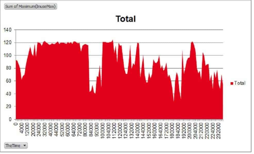
The system allows for a maximum of 120 AWTs per AMP, with a default limit of 80.

Flow control starts with the worker tasks themselves: what an AMP worker task is and what happens when they run out.

Write Ahead Logic (WAL)

Accessing data has always been the bottleneck of database systems. Once the data resides in the main memory, it can be promptly processed.

Although SSDs are now predominantly used instead of hard disks, copying data into the main memory remains the slowest operation.

The Teradata Write-Ahead Logging (WAL) feature enhances DML performance and boosts data security.

All of this sits on top of the shared-nothing architecture Teradata is built on.

Identity Columns and Their Limits

Teradata Identity Columns and CREATE TABLE AS

Facing hurdles with the Teradata Identity columns and Volatile Tables? Buckle up because we’re about to overcome this challenge. Despite the inherent limitation, there’s a clever workaround that lets you leverage the ‘CREATE TABLE AS’ statement to generate Volatile Tables, even with Identity columns. So, stick around as we unpack this ingenious solution together!

The Test Setup

Let’s dive in and start with our experimental setup. This will provide a firm groundwork for understanding the solution:

CREATE MULTISET TABLE DB.IDENTITY_TABLE (
      PK INTEGER GENERATED BY DEFAULT AS IDENTITY
         (START WITH 1
          INCREMENT BY 1
          MAXVALUE 1000000
      ),
      VAL INTEGER) PRIMARY INDEX (PK);

INSERT INTO DB.IDENTITY_TABLE (PK,VAL) VALUES (NULL,1);

To begin, we’ll establish a basic test table with an Identity column and insert a single row. This minimal setup will perfectly demonstrate our workaround when it comes to employing the ‘CREATE TABLE AS’ statement in conjunction with an Identity column.

If we proceed to replicate this table utilizing the ‘CREATE TABLE AS’ statement, we’re met with an error:

CREATE VOLATILE TABLE COPY_OF_IDENTITY_TABLE
AS
(
                SELECT PK,VAL
                FROM DB.IDENTITY_TABLE
) WITH DATA PRIMARY INDEX (PK) ON COMMIT PRESERVE ROWS;

CREATE TABLE Failed.  [5788] CREATE TABLE AS currently does not support Identity Columns.

Fortunately, a simple yet effective workaround to this issue is to conceal the Identity column by enveloping the logic within a subquery. The following example illustrates this approach:

CREATE VOLATILE TABLE COPY_OF_IDENTITY_TABLE
AS
(
    SELECT PK,VAL FROM (
    SELECT PK,VAL
    FROM DB.IDENTITY_TABLE
    ) t01
) WITH DATA PRIMARY INDEX (PK) ON COMMIT PRESERVE ROWS;

CREATE TABLE completed. 0 rows processed. Elapsed Time = 00:00:01

As demonstrated, this enhanced SQL statement enables us to leverage the ‘CREATE TABLE AS’ statement effectively, even when the source table incorporates a Teradata Identity column.

Should you have concerns that this workaround might introduce performance overhead, rest assured there is absolutely no disparity in the execution plan. Thanks to the intelligence of the Optimizer, it recognizes that the subquery can be optimized effectively. To illustrate this, let’s compare the execution plans of both queries. As you will observe, they are identical, affirming that the workaround is efficient:

Execution Plan of the Original Query

EXPLAIN
SELECT PK,VAL FROM DB.IDENTITY_TABLE;
 1) First, we lock DB.IDENTITY_TABLE in TD_MAP1 for read on a
     reserved RowHash to prevent global deadlock.
 2) Next, we lock DB.IDENTITY_TABLE in TD_MAP1 for read.
 3) We do an all-AMPs RETRIEVE step in TD_MAP1 from
     DB.IDENTITY_TABLE by way of an all-rows scan with no  residual conditions into Spool 1 (group_amps), which is built  locally on the AMPs.  The size of Spool 1 is estimated with low     confidence to be 216 rows (6,264 bytes).  The estimated time for this step is 0.02 seconds.
  -> The contents of Spool 1 are sent back to the user as the result of statement 1.  The total estimated time is 0.02 seconds.

Execution Plan of the Modified Query

EXPLAIN
SELECT PK,VAL FROM (SELECT PK,VAL  FROM DB.IDENTITY_TABLE  ) t01
1) First, we lock DB.IDENTITY_TABLE in TD_MAP1 for read on a
     reserved RowHash to prevent global deadlock.
2) Next, we lock DB.IDENTITY_TABLE in TD_MAP1 for read.
3) We do an all-AMPs RETRIEVE step in TD_MAP1 from
     DB.IDENTITY_TABLE by way of an all-rows scan with no  residual conditions into Spool 1 (group_amps), which is built  locally on the AMPs.  The size of Spool 1 is estimated with low     confidence to be 216 rows (6,264 bytes).  The estimated time for this step is 0.02 seconds.
  -> The contents of Spool 1 are sent back to the user as the result of statement 1.  The total estimated time is 0.02 seconds.

Conclusion

In conclusion, the challenge of creating Volatile Tables from tables with Identity columns in Teradata may seem daunting, but as we’ve explored, it’s far from insurmountable. With ingenuity, we’ve successfully utilized a simple subquery to hide the Identity column, effectively allowing us to use the ‘CREATE TABLE AS’ statement.

Moreover, we’ve dispelled any concerns regarding potential performance overhead. By comparing the execution plans of our original and modified queries, we found them to be identical, proving the efficiency of our workaround.

So, the next time you encounter this common Teradata hurdle, remember this clever strategy. It’s another example of how creativity can help us navigate and overcome even the most complex technical challenges. Happy querying!

For more insights on Identity columns, refer to the following article:

https://dbmstutorials.com/random_teradata/teradata-identity-column.html

Secure Zones

Teradata Secure Zones

I’ve had a few conversations recently with different customers about the “Secure Zones” optional feature added in Teradata 15.10. There is a fair amount of misunderstanding about what this feature offers and does.

This article aims to provide some clear information for anyone considering using this feature.

Before I cover that, let me describe the basic setup of Secure Zones on a Teradata system and what they offer different from previously available.

The Basics

A “Secure Zone” on a Teradata system typically contains multiple databases and users under a single database or user (referred to as the ‘root’ of that zone). The users defined in a zone can only access data in tables/views set in that zone.

A Teradata system has multiple “secure zones”, perhaps named ‘UK’ and ‘EU,’ then users in the ‘UK’ zone cannot see data in the ‘EU’ zone and vice-versa. All of this could be achieved entirely simply using standard Teradata Access Rights.

The difference that “Secure Zones” provides is that users in the UK’ zone don’t know that the ‘EU’ zone objects even exist – even if they run a query such as:

SELECT databasename,tablename,tablekind

FROM DBC.Tablesv

WHERE databasename <> ‘DBC’

ORDER BY 1,2;

In a “Secure Zones” environment, this query will not return any objects defined in the ‘EU’ zone – the’ UK’ user doesn’t even know the ‘EU’ zone or its objects exist.

The above ‘works’ because when the query is sent to the Teradata system, the SQL is effectively changed to view DBC.TablesV_SZ (and not DBC.TablesV as coded). It is this view that uses the new table DBC.Zones to filter the returned data.

There are two things to note about this mechanism:

1. This change to the SQL only happens for non-DBC users. If user DBC runs the above query, then the SQL is not modified, and rows are returned from all zones.
2. This switch to SQL only happens if it references the views (e.g., DBC.TablesV). If the SQL references the underlying tables (e.g., DBC.Dbase, DBC.TVM, etc.), no changes to the SQL are made, and rows for objects in all zones will be returned – regardless of which zone the user running this SQL is defined in.

Possible Use Case

A commonly quoted use case for the “Secure Zones” feature is where a multi-national organization needs to separate data for its different country organizations. This separation may be for regulatory requirements.

In this scenario, each country may have a separate secure zone containing databases, tables, users, etc. The data and users within each zone are specific to a country.

Assume an ‘Orders’ table exists in each zone, possibly with the exact definition. The ‘Orders’ table in each zone is a different physical table – because they are in different databases.

Therefore if there is a requirement to produce a ‘corporate-level’ Orders report spanning multiple countries (i.e., zones), the SQL has to reference various tables. Yes, that element may be hidden inside a view, but the underlying processing still requires access to various tables. Whether those tables are joined or UNION’d together is a different question and relies on the business requirement. Either solution will likely provide slower performance than all of the data in a single physical table.

Alternative Strategies

Similar data segregation (from different countries) can be achieved without using “Secure Zones,” different approaches have advantages and disadvantages.

1. Use different databases and user hierarchies for each country: This is the closest to the “Secure Zones” feature in that the data is separated into different physical tables. Access Rights can be granted such that only the appropriate users can access the data, and corporate-level reporting requires access to multiple tables. The significant difference with this approach is that a ‘UK’ user who runs the query shown above will see that the ‘EU’ objects exist.
2. Row-Level Security: With this method, only one corporate-wide Orders table (as an example) contains the data for all countries. Additional ‘row level constraint’ column(s) are added to the table definition, which causes the correct data to be returned to each user based on their access constraints (i.e., country). Corporate-level reporting now only has to access a single table.
3. Country-Specific Views: Historically, in Teradata, this has been a widespread solution to this type of requirement. The ‘Orders’ data is stored in a single physical table. A series of ‘country-specific’ views are defined, each with an appropriate WHERE clause such that only data for a particular country is returned. A user is given access to a consistent view of their country.
4. Security Table: Alternatively, a single view joins a ‘security table’ that identifies which country the user should see data.

Whether any alternate strategies provide sufficient data security for an organization is a separate question and the only one the organization can answer.

Data Encryption

The data in a “Secure Zone” table is not encrypted; it is stored like any other data in the Teradata DBMS. If you need your data encrypted, look at some Teradata partner offerings to achieve that.

Performance

The “Secure Zones” feature is not expected to enhance ETL or query processing performance. As stated above, it is possible for some processing (i.e., corporate-level reporting) to suffer in this environment.

Query Logging

These rules are unique to the user’s zone (assuming it is not DBC), executing the BEGIN / REPLACE QUERY LOGGING command.

Workload Management

Because all zones are on the same physical Teradata platform, they are all subject to the same set of rules. (I think this is one area where future versions of the Teradata DBMS software will change).

Summary

In my opinion (and it is just that), the “Secure Zones” feature is aimed at an organization that wants to offer customers a ‘cloud bureaux service’ so that those customers can take advantage of the Teradata features without having to invest in their system. Such customers will end up sharing a physical Teradata system with other independent organizations without being aware.

Please don’t get me wrong; the above requirement is not ‘bad’. It is just (in my opinion) particular, and I don’t think many organizations will have a real need for it.

Teradata in the Cloud

Add Snowflake, BigQuery, and Redshift to your Knowledge

As a passionate Teradata expert, I have fine-tuned thousands of SQL queries throughout my professional journey. It was an enjoyable and fulfilling experience to witness how, with expertise, query runtimes could be optimized from hours to mere minutes or seconds. While end-users were pleased with the results, it was challenging to quantify the cost savings resulting from such significant accomplishments.

If you know Teradata, learning Redshift, Snowflake, BigQuery, etc. is ridiculously easy.

We are currently in the era of cloud computing, with the data warehousing market being dominated by the three major players: Google, Amazon, and Microsoft. The exciting narrative of “No more performance issues, just scalability” is somewhat accurate. The marketing was also truthful: “We require no tuning, indexes, or additional components. We scale, and that’s it.”

Is everything too good to be true? I would say yes — if finances are not a concern, then it may be plausible.

Using Snowflake as an example, I admire its remarkable attributes, primarily its zero-copy cloning ability.

Disillusionment arises due to costs. Need faster query results? Scale up and pay. Want greater concurrency? Create a new warehouse and pay for it.

Conventional tuning methods like clustering or partitioning and search optimization services (referred to as indexes in Snowflake marketing) are once again pertinent. Notably, the latter has an extra charge, similar to the current pricing methods employed by car manufacturers that provide monthly rentals for parking heater functionalities.

As a performance tuner, it is clear that new opportunities are emerging regardless of personal opinions. For instance, reducing the query runtime from 30 to 1 minute can save a company a significant amount if Snowflake charges per minute.

I will continue supporting Teradata throughout my career while prioritizing other technologies such as Snowflake, Redshift, and BigQuery. These alternatives present profitable opportunities in the current market, and I am eager to take on migration and optimization projects.

A Warning About the 16.20 Upgrade

There are some important considerations to keep in mind when upgrading to Teradata 16.20.

After upgrading to Teradata 16.20, we noticed that certain reporting queries produced inconsistent result sets upon each execution. Occasionally, the results were accurate, while at other times they were inaccurate.

Upon analysis, I found a correlation between Incremental Planning and Execution (IPE). When this function is enabled, the execution plan may encounter errors. I will conduct additional research and provide an update regarding this matter. It is possible that a patch has already been released. Your feedback is welcome.

Ever since disabling this feature, my result sets have been consistently accurate. To ensure this remains the case until a resolution is found, I am implementing the following query band as a pre-SQL step on every Microstrategy report.

SET QUERY_BAND = ‘DynamicPlan=OFF;’ FOR SESSION;

This information could be helpful to those encountering this issue.

Teradata Express: Moving Between Hypervisors

The Teradata Express Edition is a great opportunity to experiment with a fully functional Teradata system. It can be downloaded from https://downloads.teradata.com/download/database.

Unfortunately, only VMware is supported as the virtualization software. As a user of Oracle’s VirtualBox, I looked for a way to convert VMware images into VirtualBox images.

After unpacking the zip file containing the Teradata Express Edition 14.10, you will find the three files needed by VMware:
sda.vmdk, PDISK0.vmdk and PDISK1.vmdk
Changing the file format from VMware to VirtualBox is relatively straightforward. The conversion process was tested with VirtualBox 4.3.10.

Follow these steps:

– Open a Windows shell (run the cmd command)
– Change the current directory to where your VirtualBox software is installed. In my case, this is:

cd C:Program FilesOracleVirtualBox

Run the conversion program from your VirtualBox installation. Be sure to convert both the Linux installation and the two virtual disks (VDISKs). The {PATH} variable must point to the directory where the Teradata Express Edition files were extracted.

VBoxManage {PATH}sda.vmdk  {PATH}sda.vdi –format VDI
VBoxManage {PATH}PDISK0.vmdk  {PATH}PDISK0.vdi –format VDI
VBoxManage {PATH}PDISK1.vmdk  {PATH}PDISK1.vdi –format VDI

These commands generate VirtualBox images that can be added directly to VirtualBox. Note that the converted images are significantly larger than the original VMware images. In my case, the original files were roughly 11 GB; after conversion, they totaled over 31 GB.

After this conversion, I successfully installed Teradata Express Edition 14.10 on VirtualBox.

Please don’t hesitate to ask if you have any questions about the conversion and installation process.

Two component-level views sit underneath all of this: a walk through the parts of a Teradata system and what sparse maps change about data distribution.

Four mechanisms underneath this are covered on their own: what the transient journal writes during a transaction, the lock levels and what each one blocks, a short tour of the architecture and the limits of identity columns in practice.

Four component-level articles: what the AMP, PE and BYNET each do, what sits inside a single node, reading object storage with NOS and how map-reduce compares with a parallel database.

Three further system-level subjects: the access paths available to the optimizer, what fallback protection costs and buys and how the pieces of a system fit together.