Teradata Physical Design and Data Modelling

Most Teradata performance problems are designed in long before anyone writes the query. This guide collects the physical design material from this site — the data model, the staging and preparatory layers, partitioning choices, and the MAPS feature — into one reference, starting with the mistakes that cause the most damage.

Seven Sins That Destroy a Teradata Data Warehouse

To exemplify the impact of mistakes in Teradata Data Warehouse projects, consider the analogy of a medical team. Imagine yourself as the project, preparing for a crucial and costly procedure. Naturally, you wouldn’t want to hear the staff engage in the following conversations before administering the anesthesia.

1. Not knowing or losing Sight of the Strategic Business Objectives

“Does anyone know why we operate on the patient? Well, let’s start anyway …”

Most Data Warehouse projects start with a lot of enthusiasm but fail in the end because they did not meet the business objectives. Very well-designed Data Warehouses will fail if the content doesn’t help to solve any business needs. Even if you see yourself as a technician first or are in a position without contact with users of the final product, never forget that whatever you produce, the customer must be satisfied.

2. Forgetting to set up Measures to evaluate the Success

“Anyone feels like this treatment is successful so far? Can we find out? No ideas? “(silence).

Even if you know your business objectives, this alone does not guarantee success. Every clear business objective is measurable. If you can’t quantify, you will have a tough time commenting on your expenses and show up on top of the blacklist as soon as the subsequent restructuring occurs. The latter usually revolves in cycles of about 3 to 5 years in length.

3. Running a Teradata Data Warehouse Project like a Mass Production via an Assembly-Line

“We need one nurse for every swab and one class-2 middle belly doctor for the first opening cut. Then, the inhalation support technicians, please stand to the right and the exhalation support professionals to the left. Is our scalpel-holding team ready?”

Overspecialization has become an enormous problem in today’s Data Warehouse projects. Industries with a more extended history are aware of the adverse effects of the extreme division of labor (look up “Taylorism”). Think of the Kaizen idea that became famous in the 80s and 90s – it seems to be the case that Data Warehousing is about to repeat history.

Any environment where each project member has to contribute to a very narrow range of skills, lacks understanding of the big picture, or is not expected to develop is predestined for failure.

It is very fashionable these days to create ever more exact roles to cut costs – at least at the beginning of a project. From my experience, this never actually pays off.

It just moves the costs from the beginning to the end of the project while they multiply along the way, and it is when you have to hire actual data warehouse experts to get back on track again. Be wary of so-called experts without real-world, hands-on experience.

4. Aiming for a Data Warehouse but achieving an Operational Data Store

“Let us just continue with aspirin and a little massage.”

While it seems tempting, from a cost perspective, to pick up the source data and provide it without any costly transformations to the customer  – even developers with no or only a little knowledge about data warehousing can be employed to do this, once again, this is the recipe for failure. I cannot overemphasize how important the implementation of a theoretically sound data model is.

Don’t even think about leaving out surrogate keys, taking over the source system-specific naming conventions, or trying to solve the issues caused by the mentioned ODS approach in the next place, like in the data marts or reports.

5. Omitting important Roles in the Teradata Data Warehouse Setup

“Why not leave out the surgeon and the anesthesiologist and ask the ambulance driver and the caretaker to help the nurse a little?”

The usual approach nowadays seems to be to leave out essential roles from the data warehouse. Never forget: Data Warehousing is a process, not a sequence of stand-alone projects. Positions that are regularly cut include:
Data Warehouse Architect, Data Modeler, Performance Specialists, or any system-specific technical experts (Teradata experts).

The typical project team consists of some highly specialized database developers missing the big picture and a project manager without academic and hands-on experience in Data Warehousing. This shortage often accompanies a lack of good relations with business departments or even fundamental project management skills. Without the support of a technical lead (Teradata expert), which can take over the roles of the architect and the general modeling of the solution, project delays, and failure are most likely.

6. Not understanding the Target Architecture and involved Tools

“Why should there be any complication? Just slice, rip, and sew!”

We should never forget that data warehousing is a very technical topic at the end of the day. The technical component is all too often considered a low-prestige subsidiary location.

The solid education of the people involved is required at many levels. In-depth knowledge and fluency are needed in Teradata, ETL-Tools (Data Stage, Informatica, Ab Initio), and Reporting Tools (Cognos, Business Objects, Microstrategy).

Too often, these different technical components’ interaction is not getting enough attention, and performance is almost always entirely ignored at the beginning of the project. Usually, omitted clarification of professional interaction and compatibility of various software can’t be handled anymore at a later time. One ends up in a minefield of workarounds upon workarounds and never-ending issues around new releases that soon start to lead a life of their own.

7. Budgetary Dishonesty and an Atmosphere of Dissimulation

“What do you mean by no vital signs? It says “operation successful” on my slide! “”

The first mile on the highway to disaster always looks perfect. It appears to be brand-new. There is no speed limit, all traffic lights are green, and you seem to drive a racing car. This part of the journey ends after the first turn.

First, suppose you start a project with amounts, assumptions, or milestones that are illusory or grossly out of touch with the average experience of professionals. In that case, it does not matter if, but only when, you see yourself in unpleasant meetings, bending over backward to add reality to the plan.

Second, if the company shows a distaste for straightforwardness, clarity, transparency, and decisiveness, not only will the real problems multiply, but alongside them, the bureaucratic dissimulation tactics will take over more and more of the remaining resources.

Your best project members are usually the first to exit this race to the bottom for better opportunities.

Why the Data Model Decides Performance

Welcome to the second part of the Teradata performance optimization series. In this session, we will examine a primary culprit responsible for performance problems in a Teradata Data Warehouse system (though it likely applies to any Data Warehouse).

A sound data model can prevent potential performance problems in the early stages of a Data Warehouse project.

Most projects fail or are subpar due to clients with budget constraints. A well-designed data model requires investment but may not yield immediately visible outcomes.

Skilled data modelers are rare. Hiring a developer proficient in efficiently loading data into the database is more cost-effective than employing a data modeler who merely draws diagrams.

The appeal of this approach lies in the prompt availability of initial outcomes and the lower cost of employing developers compared to other positions within the data warehouse job hierarchy. In a short period of time, you can deliver favorable results for your client, which will lead to their satisfaction and confidence that their investment has not been wasted.

During the global economic downturn, the data warehousing sector required a marketing term to describe the decreased quality approach caused by daily rate reductions.

Prototyping was the new buzzword.

While prototyping is a good idea in principle, it often becomes the final solution. Prototypes were originally intended as a communication tool between customers and a base for requirement specification and further analysis. However, they frequently become both the final solution and a dead end.

Making direct changes to the source definitions of operational systems during the modeling process is perhaps the most ill-advised decision that could be made.

Integrating source systems 1:1 leads to operational data stores but has nothing to do with data warehousing. Combine this with the waiving of surrogate keys, and you can be sure that sooner or later, a source system will be replaced by another one. At that point, a cost-intensive redesign will be waiting for you.

The costs of the project have been postponed and are likely to be significantly higher than the initial expenses incurred by hiring a skilled data modeler.

Regrettably, this is the era in which we exist, and we must find a way to cope with this circumstance.

I chose to withdraw from participating in substandard data warehousing projects. My recommendation is to adopt the same approach — abstain from competing with others for diminishing daily rates. Instead, wait for unsuccessful ventures to be brought to you.

The following part in this series will explore options for repairing a flawed data model.

Declared relationships are part of that model: what referential integrity tells the optimizer.

Layer and Preparatory Table Strategies

Typically, query tuning involves altering the composition of various objects.

An alternative method for achieving quicker results, in cases where modifying SQL, is not feasible or has already been completed, involves substituting the objects from which data is retrieved. By incorporating intermediate objects into a daily job chain, numerous queries can be expedited, resulting in a net increase in speed.

Here are some options for object-based query tuning that worked well for us.

Usage of volatile tables

When your first query has subqueries that need to be created several times for structurally equivalent row sets, summarize these subqueries into one and define a volatile table with the result set. Large, skewed, or otherwise “bulky” data sets can be preselected and stored independently of well-running query parts. Reference the volatile table when the subset is needed. You can index and partition your volatile table independently of source table settings. Furthermore, any preparatory row operation, such as substrings or mathematical operations on source columns, can be materialized into the volatile table and become subject to indexation or partitioning.

Regular loads  with layer tables

If you retrieve a subset of data defined similarly, consider creating layer tables first. They are structurally identical copies of source tables, only with a fraction of the original data volume. For example, if you need to work on the most recently loaded rows of your source tables and this fraction is small compared to the entire table content, create a table identical to the source table and load the fraction into it first. You can re-index or repartition if needed. Collect statistics on your layer table and adapt your SQL accordingly.

We create layer tables as normal physical tables instead of volatile ones because they will be reused by many queries or stored procedures in a row so that more than one session could be involved.

We used this strategy to cut down the average daily load time from 6 hours and more to 5 hours. Note that this net change includes the extra runtime for the layer table buildup and statistics collection on them!

Tailored auxiliary tables

We call an auxiliary table any user-defined extra table that serves other needs than holding a  row layer of data from the source tables.

When filtering data from large tables based on LIKE or NOT LIKE conditions containing a lot of non-adjacent code or value enumerations, you can create a volatile reference table with just these codes and transform the (NOT) LIKE search into a join condition on the volatile table. By this, cet. par. You enable Teradata to move to the right set of values faster.

The mechanics of the tables used for this are covered separately in how volatile tables behave, and what they cost.

Stage Table Design for Faster Loads

While stage tables are temporary objects for intermediate data, a well-designed table can distinguish between a high-performing load and a slow one. The extra effort pays off quickly.

Selecting appropriate data types and sizes is crucial. The load process inserts bytes into Teradata, impacting the load time. Optimizing the load process involves choosing the appropriate loading utility and minimizing the data volume.

Consider utilizing Multivalue compression and NoPi tables as beneficial tools.

Improper data types can significantly increase load times. In this example, we load a file twice into Teradata using fast load. The difference is that the first load defines the textual columns as CHAR, while the second load defines them as VARCHAR.

The average length of each column (COl1 to COl10) is short. Using CHAR columns is inefficient as they are filled with unnecessary spaces.

Using CHAR(1000) as the data type for all columns results in a fast load duration of over 10 seconds for every 100,000 rows.

CREATE SET TABLE DB.CHAR_TABLE
(
COL1 CHAR(1000),
COL2 CHAR(1000),
COL3 CHAR(1000),
COL4 CHAR(1000),
COL5 CHAR(1000),
COL6 CHAR(1000),
COL7 CHAR(1000),
COL8 CHAR(1000),
COL9 CHAR(1000),
COL10 CHAR(1000)
PRIMARY INDEX (COL1);

**** 19:10:05 Number of recs/msg: 10
**** 19:10:05 Starting to send to RDBMS with record 1
**** 19:10:19 Starting row 100000
**** 19:10:32 Starting row 200000
**** 19:10:49 Starting row 300000
**** 19:10:59 Starting row 400000
**** 19:11:02 Finished sending rows to the RDBMS

Using the VARCHAR(1000) data type significantly improves fast load performance, with an impressive rate of only 1 second per 100,000 rows.

CREATE SET TABLE DB.VARCHAR_TABLE
(
COL1 VARCHAR(1000),
COL2 VARCHAR(1000),
COL3 VARCHAR(1000),
COL4 VARCHAR(1000),
COL5 VARCHAR(1000),
COL6 VARCHAR(1000),
COL7 VARCHAR(1000),
COL8 VARCHAR(1000),
COL9 VARCHAR(1000),
COL10 VARCHAR(1000)
)
PRIMARY INDEX (COL1);

**** 19:20:28 Number of recs/msg: 10
**** 19:20:28 Starting to send to RDBMS with record 1
**** 19:20:28 Starting row 100000
**** 19:20:29 Starting row 200000
**** 19:20:29 Starting row 300000
**** 19:20:30 Starting row 400000
**** 19:20:31 Finished sending rows to the RDBMS

Changing the data type improved the load speed by 10x.

The efficient table design is crucial for handling wide rows as they decrease the number of rows fitting into each data block. This, in turn, leads to increased load times as IO operations are expensive.

Block size matters here too – how the data block size affects load and scan performance.

Row Partitioning for Tactical Workloads

Teradata is commonly used for tactical workloads and OLTP applications in my projects. However, it is crucial to avoid designing databases carelessly. Teradata excels as a database for strategic data warehousing.

High-performance queries can often be achieved without special design techniques. Keeping statistics current and correctly designing row partitioning is typically sufficient, while other indexes may not be frequently utilized. In terms of administration effort, strategic workloads require minimal attention. This article will provide guidance for designing Teradata Row Partitioning specifically for tactical workloads.

Teradata Row Partitioning and Tactical Workload

Row partitioning is not a means to optimize a PDM for the tactical workload, but it does facilitate queries by substituting full table scans with partition scans.

For tactical workloads, Row Partitioning should be designed to ensure peak performance.

Influence of the Design on the Performance

Row partitioning for tactical queries should use partitioning columns in the WHERE condition to access rows directly, avoiding partition probing. The customer table can be accessed in three ways, with option three offering the same performance as option one (for NPPI tables). Option two should be avoided due to partition probing.

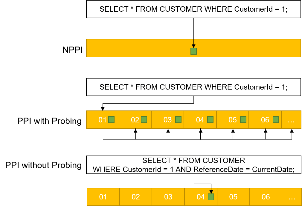
Row Partitioning Recommendations for Tactical Queries

If Primary Index Access for PPI Tables is used for tactical queries, you should consider the following:

• If possible, the PI should be unique
• The partitioning columns should be part of the Primary Index definition

Fulfilling these two conditions ensures PI rows can be located within a single partition.

If the primary index cannot include the partitioning column, it must be added to the WHERE conditions to avoid probing.

Creating a Unique Secondary Index (USI) on the Non-Unique Primary Index (NUPI) columns of the PPI table can prevent probing even if the values are unique. The USI is directly queried, and the base table’s ROWID is utilized to locate each row directly, thus circumventing the more expensive partition probing.

Moving Tables with Teradata MAPS

The Teradata MAPS Feature enables hardware configuration expansion with minimal downtime by postponing the redistribution of tables from old to new AMPs. This is achievable due to coexisting multiple hash maps that cover old and new configurations. The administrator can determine when to transfer tables to the new hash map.

Traditional INSERT…SELECT

After transitioning to a bigger hash map in Teradata, it is necessary to eventually distribute the rows of a table to the proper AMPs based on the new hash map. One effective method is utilizing a conventional INSERT-SELECT statement, which transfers the rows from the source table to a new table and redistributes them to the appropriate AMPs.

The retrieval step reads the source table, redistributes its rows, and constructs a spool file. The merge step then inserts the rows into the new table. Before dropping the initial table, removing any defined join index is mandatory.

The INSERT-SELECT statement is optimized and efficient for distributing rows after upgrading to a larger hash map in Teradata. However, an even better approach exists.

MAPS INSERT…SELECT

To transfer a table from an outdated map to a new one in Teradata, you can use an ALTER TABLE statement specifically designed for this purpose. Include a MAP = name clause. This statement operates similarly to the conventional INSERT-SELECT statement, but with some distinctions.

ALTER TABLE mytable
MAP = mynewmap;

Comparing both strategies

To transfer a table between hash maps, use an ALTER TABLE command with the MAP = mynewmap clause. This approach differs from an INSERT-SELECT statement.

The table rows persist while the owning AMP of each row changes in the new hash map due to a greater number of AMPs. Note that no tables are eliminated during the relocation of a table to a new map, unlike with the INSERT…SELECT process.

A new internal copy of the table is created, maintaining the original table entry and its Table ID in the TVM table. The rows are then read, redistributed, and inserted into a work table that replaces the original table.

The same applies to subtables. It is well-known that subtables contain Secondary indexes. When transferring a table to a different map, a task subtable must be generated for each current subtable. Every subtable is assigned a distinctive identifier that holds significance internally. Upon reaching the END TRANSACTION phase, the initial subtables are deleted, and the task subtables are renamed with the original subtable identifier.

Why should you use the MAPS approach?

Moving tables between maps does not involve row-level transient journaling, nor does it require creating a spool file. Additionally, minimal administrative intervention is necessary. An advantage of this method is that join indexes do not need to be dropped as they would with the INSERT…SELECT approach.

In the event of an error during the MAPS approach, the original tables will remain accessible and will be reverted to.

Stored Procedure Tuning with MAPS

Occasionally, it is necessary to utilize a cursor within a stored procedure to execute specific functionality. I recently encountered a stored procedure that contained a loop with multiple INSERT statements executed through a cursor. This particular cursor was designed to process only a limited number of rows. Despite this, the stored procedure took up to 6 hours, depending on the system’s current load.

In this case, a recursive or window function could have been used for a more efficient solution. However, the presented logic was convoluted and reverse engineering would have been too time-consuming due to a lack of clear specifications.

The stored procedure’s cursor utilized multiple volatile tables. I inferred that it should be possible to enhance performance by localizing the work for this limited amount of data.

The objective was twofold: consolidate the work onto a single AMP to circumvent utilizing ROWHASH for data distribution, and store the data in primary memory, which proves unchallenging for a quantity of several thousand rows.

I opted to use Teradata’s MAPS feature.

I created all volatile tables on a single AMP map to consolidate the rows into one AMP and increase the likelihood of caching or main memory storage.

CREATE TABLE DWHPRO.LocalizedWork, MAP=SingleAMP_Map
(a1 INTEGER, b1 INTEGER) UNIQUE PRIMARY INDEX (a1);

The stored procedure modification significantly decreased the runtime from six hours to just a few minutes.

I trust I have presented you with an additional instrument to aid performance optimization. Occasionally, a slight alteration can bring about a significant enhancement. Before devising the MAPS Architecture concept, I spent numerous hours attempting to comprehend the difficulty that the stored procedure aimed to rectify. Regrettably, due to the code’s lack of specifications or documentation, I eventually had to concede defeat.

Table type is part of the physical design too: what SET and MULTISET actually cost on insert.

The individual design choices have their own articles: how a partitioned primary index is defined, choosing a partitioning scheme, what partitioning does to insert performance, the primary AMP index and when it helps and why row size decides how many rows fit in a block.

Three more design decisions with their own walkthroughs: the access paths the optimizer can choose from, covering both sides of a relationship with a join index and tuning a partitioned table.

Three more structures to weigh up: soft referential integrity and join elimination, when the optimizer picks a nested join and what a hash index gives you over a join index.