
The cheapest Teradata tuning available is almost never a new index. It is rewriting the query so the optimizer has less work to do and better information to do it with. This guide gathers the query-rewriting material from this site into one place: full worked examples first, then the individual operators and patterns that repeatedly cause trouble.
How Query Rewriting Reduces Resource Usage
It’s time to share a new Teradata SQL tuning case study that showcases the impressive impact of query rewriting on performance.
We are studying the query below that originally took 40 minutes to run.
As a SQL tuning specialist, I always prioritize adding missing statistics and refreshing stale ones.
I analyzed the SQL statement that generates a call detail report for a telecom company and selects the total minutes of use (MOU) for a specific day.
CALL_DATE partitions the call detail (CDR) table, and I expected partition elimination when using the CALL_DATE as a predicate of the WHERE condition.I discovered an execution step that implemented partition elimination but was not executed optimally. It involved a product join with the large call detail table, which was improved by dynamic partition elimination.
Upon further analysis, I discovered that the Optimizer filtered call detail records at the end of the execution plan via the HAVING clause.
Moving the CALL_DATE filter to the driving table’s WHERE condition enabled the Optimizer to apply static partition elimination at the start of the execution plan.
This minor adjustment decreased the query’s execution time to mere seconds, while the initial query took 40 minutes to complete.
An authentic Teradata SQL Tuning Home Run
Conclusion:
Optimize data retrieval by applying filters as early as possible in the SQL statement, particularly on the driving table, to ensure efficient execution. Despite the optimizer’s capabilities, it may not identify all potential opportunities. Poorly performing query:
SELECT
TOT.PHONE_ID
, TOT.COUNTRY_CD
, TOT.BILLING_ENGINE_CD
, TOT.PRICEPLAN_GROUP_CD
, TOT.RATING_CODE
, TOT.CUSTOMER_ID
, TOT.REPORTING_GROUP_CD1
, TOT.ROAMING_IND
, TOT.CORRECTIONS_IND
, TOT.CALL_DATE
, TOT.BILL_PERIOD_CD
, 'A6' AS PROVIDER_CD
, SUM(TOT.MINUTES_OF_USE) AS MINUTES_OF_USE
, TOT.BILLED_IND
, TOT.PREPAID_IND
FROM
(SELECT
RG.PHONE_ID
, RG.COUNTRY_CD
, RG.BILLING_ENGINE_CD
, RG.PRICEPLAN_GROUP_CD
, RG.RATING_CODE
, RG.CUSTOMER_ID
, RG.REPORTING_GROUP_CD1
, RG.ROAMING_IND
, RG.CORRECTIONS_IND
, RG.REPORTING_GROUP_CD2
, RG.CALL_DATE
, RG.BILL_PERIOD_CD
, RG.MINUTES_OF_USE
, RG.BILLED_IND
, RG.PREPAID_IND
FROM
(SELECT
CD.PHONE_ID
, CD.COUNTRY_CD
, CD.BILLING_ENGINE_CD
, CD.PRICEPLAN_GROUP_CD
, CD.RATING_CODE
, CD.CUSTOMER_ID
, CD.REPORTING_GROUP_CD1
, CD.ROAMING_IND
, CD.CORRECTIONS_IND
, CD.REPORTING_GROUP_CD2
, CD.CALL_DATE
, CD.MINUTES_OF_USE
, RG.BILL_PERIOD_CD
, CD.BILLED_IND
, CD.PREPAID_IND
FROM
CALL_DETAILS CD
LEFT JOIN
(SELECT BILL_PERIOD_CD, CALL_DATE FROM REPORTING_GROUP GROUP BY 1,2) RG
ON CD.CALL_DATE = RG.CALL_DATE
WHERE
BILLING_ENGINE_CD IN ('AMDOCS')
AND BILLED_IND = 'N'
AND REPORTING_GROUP_CD2 IS NOT NULL
) RG
LEFT JOIN
REPORTING_GROUP R1
ON RG.CALL_DATE = R1.CALL_DATE
AND RG.REPORTING_GROUP_CD1 = R1.REPORTING_GROUP_CD1
AND RG.BILL_PERIOD_CD = R1.BILL_PERIOD_CDLEFT JOIN
REPORTING_GROUP R2
ON RG.CALL_DATE = R2.CALL_DATE
AND RG.REPORTING_GROUP_CD2 = R2.REPORTING_GROUP_CD1
AND RG.BILL_PERIOD_CD = R2.BILL_PERIOD_CD
WHERE NOT (R1.REPORTING_GROUP_CD1 IS NULL OR R2.REPORTING_GROUP_CD1 IS NULL)
) TOT
GROUP BY 1,2,3,4,5,6,7,8,9,10,11,12,14,15
HAVING TOT.CALL_DATE = DATE '2015-05-21';This is the execution plan for the poorly-performing query:
1) First, we lock CALL_DB.REPORTING_GROUP for access,
and we lock CALL_DB.CALL_DETAILS for access.
2) Next, we do an all-AMPs SUM step to aggregate from
CALL_DB.REPORTING_GROUP by way of an all-rows
scan with no residual conditions , grouping by field1 (
CALL_DB.REPORTING_GROUP.BILL_PERIOD_CD
,CALL_DB.REPORTING_GROUP.CALL_DATE). Aggregate
Intermediate Results are computed globally, then placed in Spool 3.
The size of Spool 3 is estimated with high confidence to be 12
rows (612 bytes). The estimated time for this step is 0.02
seconds.3) We do an all-AMPs RETRIEVE step from Spool 3 (Last Use) by way of
an all-rows scan into Spool 1 (used to materialize view, derived
table, or table function RG) (all_amps) (compressed columns
allowed), which is built locally on the AMPs. The size of Spool 1
is estimated with high confidence to be 12 rows (444 bytes). The
estimated time for this step is 0.01 seconds.4) We execute the following steps in parallel.
1) We do an all-AMPs RETRIEVE step from Spool 1 (Last Use) by
way of an all-rows scan into Spool 8 (all_amps) (compressed
columns allowed), which is duplicated on all AMPs. Then we
do a SORT to order Spool 8 by the hash code of (
CALL_DB.REPORTING_GROUP.BILL_PERIOD_CD,
CALL_DB.REPORTING_GROUP.CALL_DATE). The size
of Spool 8 is estimated with high confidence to be 1,080 rows
(31,320 bytes). The estimated time for this step is 0.01
seconds.2) We do an all-AMPs RETRIEVE step from
CALL_DB.REPORTING_GROUP by way of an
all-rows scan with no residual conditions locking for access
into Spool 9 (all_amps) (compressed columns allowed), which
is built locally on the AMPs. Then we do a SORT to order
spool 9 by the hash code of (
CALL_DB.REPORTING_GROUP.BILL_PERIOD_CD,
CALL_DB.REPORTING_GROUP.CALL_DATE). The size
of Spool 9 is estimated with high confidence to be 4,277 rows
(149,695 bytes). The estimated time for this step is 0.01
seconds.5) We do an all-AMPs JOIN step from Spool 8 (Last Use) by way of a
RowHash match scan, which is joined to Spool 9 (Last Use) by way
of a RowHash match scan. Spool 8 and Spool 9 are joined using a
merge join, with a join condition of ("(CALL_DATE = CALL_DATE) AND
(BILL_PERIOD_CD = BILL_PERIOD_CD)"). The result
goes into Spool 10 (all_amps) (compressed columns allowed), which
is duplicated on all AMPs. Then we do a SORT to partition by
rowkey. The size of Spool 10 is estimated with low confidence to
be 384,930 rows (19,631,430 bytes). The estimated time for this
step is 0.03 seconds.6) We execute the following steps in parallel.
1) We do an all-AMPs JOIN step from Spool 10 (Last Use) by way
of an all-rows scan, which is joined to
CALL_DB.CALL_DETAILS with a condition of (
"(CALL_DB.CALL_DETAILS.BILLED_IND = 'N') AND (CALL_DB.CALL_DETAILS.BILLING_ENGINE_CD = 'AMDOCS ')").Spool 10 and CALL_DB.CALL_DETAILS are joined
using a product join, with a join condition of (
"(CALL_DB.CALL_DETAILS.CALL_DATE = CALL_DATE) AND
((CALL_DB.CALL_DETAILS.CALL_DATE = CALL_DATE) AND
(CALL_DB.CALL_DETAILS.REPORTING_GROUP_CD2 = REPORTING_GROUP_CD1
))") enhanced by dynamic partition elimination.
The input table CALL_DB.CALL_DETAILS will not be cached in
memory, but it is eligible for synchronized scanning. The
result goes into Spool 11 (all_amps) (compressed columns
allowed), which is built locally on the AMPs. The size of
Spool 11 is estimated with low confidence to be 136,515 rows
(21,159,825 bytes). The estimated time for this step is 4.15
seconds.2) We do an all-AMPs RETRIEVE step from
CALL_DB.REPORTING_GROUP by way of an
all-rows scan with no residual conditions locking for access
into Spool 12 (all_amps) (compressed columns allowed), which
is duplicated on all AMPs. The size of Spool 12 is estimated
with high confidence to be 384,930 rows (13,857,480 bytes).The estimated time for this step is 0.02 seconds.7) We do an all-AMPs JOIN step from Spool 11 (Last Use) by way of an
all-rows scan, which is joined to Spool 12 (Last Use) by way of an
all-rows scan. Spool 11 and Spool 12 are joined using a single
partition hash join, with a join condition of (
"(BILL_PERIOD_CD = BILL_PERIOD_CD) AND ((CALL_DATE
= CALL_DATE) AND ((CALL_DATE = CALL_DATE) AND
((BILL_PERIOD_CD = BILL_PERIOD_CD) AND ((CALL_DATE
= CALL_DATE) AND (REPORTING_GROUP_CD1 = REPORTING_GROUP_CD1 )))))"). The result goes into Spool 7 (all_amps) (compressed columns allowed), which is
built locally on the AMPs. The size of Spool 7 is estimated with
low confidence to be 136,515 rows (18,702,555 bytes). The
estimated time for this step is 0.04 seconds.8) We do an all-AMPs SUM step to aggregate from Spool 7 (Last Use) by
way of an all-rows scan, grouping by field1 (
CALL_DB.CALL_DETAILS.PHONE_ID
, CALL_DB.CALL_DETAILS.COUNTRY_CD
, CALL_DB.CALL_DETAILS.BILLING_ENGINE_CD
, CALL_DB.CALL_DETAILS.PRICEPLAN_GROUP_CD
, CALL_DB.CALL_DETAILS.RATING_CODE
, CALL_DB.CALL_DETAILS.CUSTOMER_ID
, CALL_DB.CALL_DETAILS.REPORTING_GROUP_CD1
, CALL_DB.CALL_DETAILS.ROAMING_IND
, CALL_DB.CALL_DETAILS.CORRECTIONS_IND
, CALL_DB.CALL_DETAILS.CALL_DATE
, CALL_DB.REPORTING_GROUP.BILL_PERIOD_CD
,'A6' ,CALL_DB.CALL_DETAILS.BILLED_IND
, CALL_DB.CALL_DETAILS.PREPAID_IND). AggregateIntermediate Results are computed globally, then placed in Spool
The size of Spool 13 is estimated with low confidence to be
102,387 rows (31,637,583 bytes). The estimated time for this step
is 0.17 seconds.
9) We do an all-AMPs RETRIEVE step from Spool 13 (Last Use) by way of
an all-rows scan with a condition of ("CALL_DATE = DATE
'2015-05-21'") into Spool 5 (group_amps), which is built locally
on the AMPs. The size of Spool 5 is estimated with low confidence
to be 102,387 rows (14,846,115 bytes). The estimated time for
this step is 0.02 seconds.10) Finally, we send out an END TRANSACTION step to all AMPs involved
in processing the request.-> The contents of Spool 5 are sent back to the user as the result of
statement 1. The total estimated time is 4.44 seconds.Here is the optimized query:
EXPLAIN
SELECT
TOT.PHONE_ID
, TOT.COUNTRY_CD
, TOT.BILLING_ENGINE_CD
, TOT.PRICEPLAN_GROUP_CD
, TOT.RATING_CODE
, TOT.CUSTOMER_ID
, TOT.REPORTING_GROUP_CD1
, TOT.ROAMING_IND
, TOT.CORRECTIONS_IND
, TOT.CALL_DATE
, TOT.BILL_PERIOD_CD
, 'A6' AS PROVIDER_CD
, SUM(TOT.MINUTES_OF_USE) AS MINUTES_OF_USE
, TOT.BILLED_IND
, TOT.PREPAID_INDFROM
(SELECT
RG.PHONE_ID
, RG.COUNTRY_CD
, RG.BILLING_ENGINE_CD
, RG.PRICEPLAN_GROUP_CD
, RG.RATING_CODE
, RG.CUSTOMER_ID
, RG.REPORTING_GROUP_CD1
, RG.ROAMING_IND
, RG.CORRECTIONS_IND
, RG.REPORTING_GROUP_CD2
, RG.CALL_DATE
, RG.BILL_PERIOD_CD
, RG.MINUTES_OF_USE
, RG.BILLED_IND
, RG.PREPAID_INDFROM
(SELECT
CD.PHONE_ID
, CD.COUNTRY_CD
, CD.BILLING_ENGINE_CD
, CD.PRICEPLAN_GROUP_CD
, CD.RATING_CODE
, CD.CUSTOMER_ID
, CD.REPORTING_GROUP_CD1
, CD.ROAMING_IND
, CD.CORRECTIONS_IND
, CD.REPORTING_GROUP_CD2
, CD.CALL_DATE
, CD.MINUTES_OF_USE
, RG.BILL_PERIOD_CD
, CD.BILLED_IND
, CD.PREPAID_INDFROM
CALL_DETAILS CD
LEFT JOIN
(SELECT BILL_PERIOD_CD, CALL_DATE FROM REPORTING_GROUP GROUP BY 1,2) RG
ON CD.CALL_DATE = RG.CALL_DATE
WHERE
BILLING_ENGINE_CD IN ('AMDOCS')
AND BILLED_IND = 'N'
AND REPORTING_GROUP_CD2 IS NOT NULL
AND CD.CALL_DATE = DATE '2015-05-21' -- The optimized place of the filter) RG
LEFT JOIN
REPORTING_GROUP R1
ON RG.CALL_DATE = R1.CALL_DATE
AND RG.REPORTING_GROUP_CD1 = R1.REPORTING_GROUP_CD1
AND RG.BILL_PERIOD_CD = R1.BILL_PERIOD_CD
LEFT JOIN
REPORTING_GROUP R2
ON RG.CALL_DATE = R2.CALL_DATE
AND RG.REPORTING_GROUP_CD2 = R2.REPORTING_GROUP_CD1
AND RG.BILL_PERIOD_CD = R2.BILL_PERIOD_CD
WHERE NOT (R1.REPORTING_GROUP_CD1 IS NULL OR R2.REPORTING_GROUP_CD1 IS NULL)) TOT
GROUP BY 1,2,3,4,5,6,7,8,9,10,11,12,14,15;Below is the optimized query execution plan:
1) First, we lock CALL_DB.REPORTING_GROUP for access,
and we lock CALL_DB.CALL_DETAILS for access.
2) Next, we do an all-AMPs SUM step to aggregate from a single
partition of CALL_DB.REPORTING_GROUP with a
condition of ("CALL_DB.REPORTING_GROUP.CALL_DATE =
DATE '2015-05-21'") with a residual condition of (
"CALL_DB.REPORTING_GROUP.CALL_DATE = DATE
'2015-05-21'") , grouping by field1 (
CALL_DB.REPORTING_GROUP.BILL_PERIOD_CD
,CALL_DB.REPORTING_GROUP.CALL_DATE). Aggregate
Intermediate Results are computed globally, then placed in Spool 3.
The size of Spool 3 is estimated with low confidence to be 4 rows
(204 bytes). The estimated time for this step is 0.01 seconds.
3) We do an all-AMPs RETRIEVE step from Spool 3 (Last Use) by way of
an all-rows scan into Spool 1 (used to materialize view, derived
table or table function RG) (all_amps) (compressed columns
allowed), which is built locally on the AMPs. The size of Spool 1
is estimated with low confidence to be 4 rows (148 bytes). The
estimated time for this step is 0.01 seconds.4) We execute the following steps in parallel.1) We do an all-AMPs RETRIEVE step from Spool 1 (Last Use) by
way of an all-rows scan with a condition of ("RG.CALL_DATE =
DATE '2015-05-21'") into Spool 8 (all_amps) (compressed
columns allowed), which is duplicated on all AMPs. Then we
do a SORT to order Spool 8 by the hash code of (
CALL_DB.REPORTING_GROUP.BILL_PERIOD_CD).The size of Spool 8 is estimated with low confidence to be
360 rows (10,440 bytes). The estimated time for this step is
0.01 seconds.2) We do an all-AMPs RETRIEVE step from a single partition of
CALL_DB.REPORTING_GROUP with a condition of
("CALL_DB.REPORTING_GROUP.CALL_DATE = DATE
'2015-05-21'") with a residual condition of (
"CALL_DB.REPORTING_GROUP.CALL_DATE = DATE
'2015-05-21'") locking for access into Spool 9 (all_amps)
(compressed columns allowed), which is built locally on the
AMPs. Then we do a SORT to order Spool 9 by the hash code of(
CALL_DB.REPORTING_GROUP.BILL_PERIOD_CD).The size of Spool 9 is estimated with high confidence to be
1,591 rows (55,685 bytes). The estimated time for this step
is 0.00 seconds.3) We do an all-AMPs RETRIEVE step from a single partition of
CALL_DB.REPORTING_GROUP with a condition of
("CALL_DB.REPORTING_GROUP.CALL_DATE = DATE
'2015-05-21'") with a residual condition of (
"CALL_DB.REPORTING_GROUP.CALL_DATE = DATE
'2015-05-21'") locking for access into Spool 10 (all_amps)
(compressed columns allowed), which is duplicated on all AMPs.The size of Spool 10 is estimated with high confidence to be
143,190 rows (5,011,650 bytes). The estimated time for this
step is 0.01 seconds.4) We do an all-AMPs RETRIEVE step from a single partition of
CALL_DB.CALL_DETAILS with a condition of (
"CALL_DB.CALL_DETAILS.CALL_DATE = DATE
'2015-05-21'") with a residual condition of ("(NOT(CALL_DB.CALL_DETAILS.REPORTING_GROUP_CD2 IS NULL ))
AND ((CALL_DB.CALL_DETAILS.CALL_DATE = DATE
'2015-05-21') AND ((CALL_DB.CALL_DETAILS.BILLED_IND = 'N') AND
(CALL_DB.CALL_DETAILS.BILLING_ENGINE_CD = 'AMDOCS
')))") into Spool 11 (all_amps) (compressed columns allowed),
which is built locally on the AMPs. The size of Spool 11 is
estimated with low confidence to be 212,693 rows (27,224,704
bytes). The estimated time for this step is 0.06 seconds.5) We do an all-AMPs JOIN step from Spool 8 (Last Use) by way of a
RowHash match scan, which is joined to Spool 9 (Last Use) by way
of a RowHash match scan. Spool 8 and Spool 9 are joined using a
merge join, with a join condition of ("(BILL_PERIOD_CD =
BILL_PERIOD_CD) AND (CALL_DATE = CALL_DATE)"). The result
goes into Spool 12 (all_amps) (compressed columns allowed), which
is duplicated on all AMPs. The size of Spool 12 is estimated with
low confidence to be 143,190 rows (7,302,690 bytes). The
estimated time for this step is 0.02 seconds.6) We do an all-AMPs JOIN step from Spool 10 (Last Use) by way of an
all-rows scan, which is joined to Spool 11 (Last Use) by way of an
all-rows scan. Spool 10 and Spool 11 are joined using a single
partition hash join, with a join condition of ("(REPORTING_GROUP_CD1 =
REPORTING_GROUP_CD1) AND (CALL_DATE = CALL_DATE)"). The result goes into
Spool 13 (all_amps) (compressed columns allowed), which is built
locally on the AMPs. The size of Spool 13 is estimated with low
confidence to be 654,535 rows (94,907,575 bytes). The estimated
time for this step is 0.11 seconds.7) We do an all-AMPs JOIN step from Spool 12 (Last Use) by way of an
all-rows scan, which is joined to Spool 13 (Last Use) by way of an
all-rows scan. Spool 12 and Spool 13 are joined using a single
partition hash join, with a join condition of ("(REPORTING_GROUP_CD2 =
REPORTING_GROUP_CD1) AND ((CALL_DATE = CALL_DATE) AND ((CALL_DATE = CALL_DATE)AND ((BILL_PERIOD_CD = BILL_PERIOD_CD) AND
((CALL_DATE = CALL_DATE) AND ((CALL_DATE = CALL_DATE) AND
(BILL_PERIOD_CD = BILL_PERIOD_CD ))))))"). The
result goes into Spool 7 (all_amps) (compressed columns allowed),
which is built locally on the AMPs. The size of Spool 7 is
estimated with low confidence to be 473,348 rows (64,848,676
bytes). The estimated time for this step is 0.10 seconds.8) We do an all-AMPs SUM step to aggregate from Spool 7 (Last Use) by
way of an all-rows scan , grouping by field1 (
CALL_DB.CALL_DETAILS.PHONE_ID,CALL_DB.CALL_DETAILS.COUNTRY_CD
,CALL_DB.CALL_DETAILS.BILLING_ENGINE_CD
,CALL_DB.CALL_DETAILS.PRICEPLAN_GROUP_CD
,CALL_DB.CALL_DETAILS.RATING_CODE
,CALL_DB.CALL_DETAILS.CUSTOMER_ID
,CALL_DB.CALL_DETAILS.REPORTING_GROUP_CD1
,CALL_DB.CALL_DETAILS.ROAMING_IND
,CALL_DB.CALL_DETAILS.CORRECTIONS_IND
,CALL_DB.CALL_DETAILS.CALL_DATE
,CALL_DB.REPORTING_GROUP.BILL_PERIOD_CD
,'TOT' ,CALL_DB.CALL_DETAILS.BILLED_IND
,CALL_DB.CALL_DETAILS.PREPAID_IND). Aggregate
Intermediate Results are computed globally, then placed in Spool
The size of Spool 14 is estimated with no confidence to be
355,011 rows (109,698,399 bytes). The estimated time for this
step is 0.32 seconds.9) We do an all-AMPs RETRIEVE step from Spool 14 (Last Use) by way of
an all-rows scan into Spool 5 (group_amps), which is built locally
on the AMPs. The size of Spool 5 is estimated with no confidence
to be 355,011 rows (51,476,595 bytes). The estimated time for
this step is 0.06 seconds.10) Finally, we send out an END TRANSACTION step to all AMPs involved
in processing the request.-> The contents of Spool 5 are sent back to the user as the result of
statement 1. The total estimated time is 0.70 seconds.A smaller but common example of the same idea is the difference between GROUP BY and DISTINCT for aggregation.
A Query Rewriting Walkthrough
Query rewriting is a potent approach for enhancing performance through row partition elimination. The following test configuration is based on an actual optimization I performed recently.
We are dealing with a straightforward query: we only want to retrieve the rows of one row partition of our test table. Nevertheless, vast improvements were possible by rewriting the query.
Our table for testing comprises approximately 400 million rows and is partitioned according to the following DDL statement:
CREATE MULTISET TABLE TheDatabase. TheTable
(
PK BIGINT NOT NULL
COL1,
…
COLn
) PRIMARY INDEX (PK)
PARTITION BY (
CASE_N(COL1 = ‘100’,COL1 = ‘200’,COL1 = ‘300’,COL1 = ‘400’,
COL1 = ‘500’,COL1 = ‘600’,COL1 = ‘700’,COL1 = ‘800’,COL1 = ‘900’, NO CASE, UNKNOWN)
);
The task is to retrieve rows where the value in the COL1 column is ‘100’. We’ll start by writing the most straightforward query:
SELECT * FROM TheDatabase.TheTable WHERE COL1 = '100';As anticipated, the execution plan comprises a single retrieval step.
The optimizer can use static partition elimination to substitute the literal value of ‘100’ when creating the execution plan.
Important note: The required statistics are readily available (“high confidence”) and up to date in our tests.
1) First, we lock a distinct TheDatabase. “pseudo table” for read on a RowHash
to prevent global deadlock for TheDatabase. TheTable.
2) Next, we lock TheDatabase. TheTable for read.
3) We do an all-AMPs RETRIEVE step from a single partition of
TheDatabase. TheTable with a condition of (
“TheDatabase. TheTable. COL1 = ‘100’”) into Spool 1
(group_amps), which is built locally on the AMPs. The input table
will not be cached in memory, but it is eligible for synchronized
scanning. The result spool file will not be cached in memory.
The size of Spool 1 is estimated with high confidence to be
108,121,098 rows (23,354,157,168 bytes). The estimated time for
this step is 18.85 seconds.
4) Finally, we send out an END TRANSACTION step to all AMPs involved
in processing the request.
-> The contents of Spool 1 are sent back to the user as the result of
statement 1. The total estimated time is 18.85 seconds.
The performance diagram below shows the optimal situation and represents our benchmark:
| Rows | Disk IOs | CPU Seconds | Spool Space |
| 108.121.087,00 | 294.425,00 | 489,64 | 20.831.922.176,00 |
Assuming a literal cannot be used for COL1, we must dynamically pass the value ‘100’ from another table into the query.
There are several ways of rewriting this query. Below is our first attempt:
(
COL1 CHAR(03) NOT NULL
) PRIMARY INDEX (COL1) ON COMMIT PRESERVE ROWS;
INSERT INTO TMP_COL1 VALUES (‘100’);
SELECT * FROM TheDatabase.TheTable WHERE COL1 IN (SELECT COL1 FROM TMP_COL1);This is the resulting execution plan:
1) First, we lock a distinct TheDatabase.” pseudo table” for read
on a RowHash to prevent global deadlock for
TheDatabase. TheTable.
2) Next, we lock TheDatabase. TheTable for read.
3) We do an all-AMPs RETRIEVE step from TheUser. TMP_COL1 by way
of an all-rows scan with no residual conditions into Spool 3
(all_amps), which is built locally on the AMPs. Then we do a SORT
to order Spool 3 by the sort key in spool field1 (
TheUser. TMP_COL1.COL1) eliminating duplicate rows. The
size of Spool 3 is estimated with high confidence to be 1 row (20
bytes). The estimated time for this step is 0.02 seconds.
4) We do an all-AMPs RETRIEVE step from Spool 3 (Last Use) by way of
an all-rows scan into Spool 2 (all_amps) (compressed columns
allowed), which is duplicated on all AMPs. The size of Spool 2 is
estimated with high confidence to be 90 rows (1,800 bytes).
5) We do an all-AMPs JOIN step from TheDatabase. TheTable by way
of an all-rows scan with no residual conditions, which is joined
to Spool 2 (Last Use) by way of an all-rows scan.
TheDatabase. TheTable and Spool 2 are joined using a inclusion
dynamic hash join, with a join condition of (
“TheDatabase. TheTable. COL1 = COL1”). The input table
TheDatabase. TheTable will not be cached in memory. The
result goes into Spool 1 (group_amps), which is built locally on
the AMPs. The size of Spool 1 is estimated with low confidence to
be 27,071,447 rows (5,847,432,552 bytes). The estimated time for
this step is 24.66 seconds.
6) Finally, we send out an END TRANSACTION step to all AMPs involved
in processing the request.
-> The contents of Spool 1 are sent back to the user as the result of
statement 1.
Initially, the table TMP_COL1 is partitioned in the same manner as “TheDatabase. TheTable” and duplicated to all AMPs. It contains a single row with the value for COL1.
A dynamic inclusion hash join is performed, without any partition elimination.
The query from our first attempt creates 197% more IOs and consumes 145% more CPU seconds when compared to our benchmark query (but the spool usage is the same):
| Rows | Disk IOs | CPU Seconds | Spool Space |
| 108.121.087,00 | 580.757,00 | 711,81 | 20.831.922.176,00 |
We need to rewrite the query to trigger partition elimination.
Here is another revised version of the benchmarking query. We are using a correlated subquery instead of the “IN (SELECT * FROM …):
SELECT * FROM TheDatabase. TheTable t01
WHERE EXISTS (SELECT COL1 FROM TMP_COL1 t02 WHERE t01.COL1 = t02.COL1);
Upon inspection of the execution plan, it is evident that there is no improvement.
Explain SELECT * FROM TheDatabase. TheTable t01
WHERE EXISTS (SELECT COL1 FROM TMP_COL1 t02 WHERE t01.COL1 = t02.COL1)
1) First, we lock a distinct TheDatabase.” pseudo table” for read
on a RowHash to prevent global deadlock for TheDatabase.t01.
2) Next, we lock TheDatabase.t01 for read.
3) We do an all-AMPs RETRIEVE step from TheUser.t02 by way of an
all-rows scan with no residual conditions into Spool 3 (all_amps),
which is built locally on the AMPs. Then we do a SORT to order
Spool 3 by the sort key in spool field1 (TheUser.t02.COL1)
eliminating duplicate rows. The size of Spool 3 is estimated with
high confidence to be 1 row (20 bytes). The estimated time for
this step is 0.02 seconds.
4) We do an all-AMPs RETRIEVE step from Spool 3 (Last Use) by way of
an all-rows scan into Spool 2 (all_amps) (compressed columns
allowed), which is duplicated on all AMPs. The size of Spool 2 is
estimated with high confidence to be 90 rows (1,800 bytes).
5) We do an all-AMPs JOIN step from TheDatabase.t01 by way of an
all-rows scan with no residual conditions, which is joined to
Spool 2 (Last Use) by way of an all-rows scan. TheDatabase.t01
and Spool 2 are joined using a inclusion dynamic hash join, with a
join condition of (“TheDatabase.t01.COL1 = COL1”). The
input table TheDatabase.t01 will not be cached in memory. The
result goes into Spool 1 (group_amps), which is built locally on
the AMPs. The size of Spool 1 is estimated with low confidence to
be 27,071,447 rows (5,847,432,552 bytes). The estimated time for
this step is 24.66 seconds.
6) Finally, we send out an END TRANSACTION step to all AMPs involved
in processing the request.
-> The contents of Spool 1 are sent back to the user as the result of
statement 1.
The following performance diagram indicates that the performance metrics remain consistent with those of the previous query:
| Rows | Disk IOs | CPU Seconds | Spool Space |
| 108.121.087,00 | 585.999,00 | 743,45 | 20.831.922.176,00 |
On the third try, I rewrote the query as a straightforward INNER JOIN.
SELECT * FROM TheDatabase. TheTable t01
INNER JOIN
TMP_COL1 t02
ON
T01.COL1 = T02.COL1;
Please find below the updated execution plan:
Explain SELECT * FROM TheDatabase. TheTable t01
INNER JOIN
TMP_COL1 t02
ON T01.COL1 = T02.COL1
1) First, we lock a distinct TheDatabase.” pseudo table” for read
on a RowHash to prevent global deadlock for TheDatabase.t01.
2) Next, we lock TheDatabase.t01 for read.
3) We do an all-AMPs RETRIEVE step from TheUser.t02 by way of an
all-rows scan with no residual conditions into Spool 2 (all_amps)
(compressed columns allowed), which is duplicated on all AMPs.
Then we do a SORT to partition by rowkey. The size of Spool 2 is
estimated with high confidence to be 180 rows (2,880 bytes). The
estimated time for this step is 0.01 seconds.
4) We do an all-AMPs JOIN step from Spool 2 (Last Use) by way of an
all-rows scan, which is joined to TheDatabase.t01 by way of an
all-rows scan with no residual conditions. Spool 2 and
TheDatabase.t01 are joined using a product join, with a join
condition of (“TheDatabase.t01.COL1 = COL1”) enhanced by
dynamic partition elimination. The input table TheDatabase.t01
will not be cached in memory, but it is eligible for synchronized
scanning. The result goes into Spool 1 (group_amps), which is
built locally on the AMPs. The size of Spool 1 is estimated with
low confidence to be 54,142,893 rows (11,857,293,567 bytes). The
estimated time for this step is 26.79 seconds.
5) Finally, we send out an END TRANSACTION step to all AMPs involved
in processing the request.
-> The contents of Spool 1 are sent back to the user as the result of
statement 1. The total estimated time is 26.80 seconds.
The execution plan for our benchmark query looks promising.
The join step utilizes dynamic partition elimination in a product join.
Knowing that the left table (TMP_COL1) has only one row, we can anticipate improved query performance compared to our previous two queries.
The FSG stores the TMP_COL1 row and compares it to the matching partition where COL1=’100′.
Therefore, the impact of the product join should be negligible, while dynamic partition elimination is expected to improve query performance significantly. In fact, the performance diagram below illustrates that we are achieving nearly identical results (with only a slight increase in CPU seconds) to the benchmark query that used static partition elimination.
| Rows | Disk IOs | CPU Seconds | Spool Space |
| 108.121.087,00 | 295.099,00 | 596,86 | 21.214.113.280,00 |
Conclusion:
Although the optimizer generally performs well, analyzing the execution plan and looking for potential improvements is beneficial. In this case, a minor query rewrite decreased disk IO by 50%.
TD_WhichMax and TD_WhichMin
What is the Teradata TD_WhichMax Function?
Teradata releases new SQL features with each update, providing enhanced functionality and improved performance with reduced resource usage.
We will examine the Teradata TD_WhichMax and TD_WhichMin functions and explore their potential benefits.
These functions retrieve the minimum or maximum value of a column and are commonly utilized in SQL using the following syntax:
SELECT * FROM DWHPRO.TESTTABLE
WHERE ID IN
(
   SELECT MAX(ID)
   FROM  DWHPRO.TESTTABLE
);
Here is the Execution Plan:
3) We do an all-AMPs SUM step in TD_MAP1 to aggregate from
     DWHPRO.TESTTABLE by way of an all-rows scan with no
     residual conditions, grouping by field1 (25570).  Aggregate
     intermediate results are computed globally, then placed in Spool 2
     in TD_Map1.  The input table will not be cached in memory, but it
     is eligible for synchronized scanning.  The size of Spool 2 is
     estimated with high confidence to be 1 row (19 bytes).  The
     estimated time for this step is 44.87 seconds.
  4) We do an all-AMPs RETRIEVE step in TD_Map1 from Spool 2 (Last Use)
     by way of an all-rows scan into Spool 6 (all_amps) (compressed
     columns allowed), which is duplicated on all AMPs in TD_Map1.  The
     size of Spool 6 is estimated with high confidence to be 216 rows (
     3,672 bytes).  The estimated time for this step is 0.01 seconds.
  5) We do an all-AMPs JOIN step in TD_Map1 from Spool 6 (Last Use) by
     way of an all-rows scan, which is joined to
     DWHPRO.TESTTABLE by way of an all-rows scan with no
     residual conditions.  Spool 6 and DWHPRO.TESTTABLE are
     joined using a product join, with a join condition of (
     "DWHPRO.TESTTABLE.ID = Field_2").  The input
     table DWHPRO.TESTTABLE will not be cached in memory,
     but it is eligible for synchronized scanning.  The result goes
     into Spool 1 (group_amps), which is built locally on the AMPs.
     The size of Spool 1 is estimated with no confidence to be 67,590
     rows (46,096,380 bytes).  The estimated time for this step is
     33.51 seconds.
  6) Finally, we send out an END TRANSACTION step to all AMPs involved
     in processing the request.
  -> The contents of Spool 1 are sent back to the user as the result of
     statement 1.  The total estimated time is 1 minute and 18 seconds.
The “TESTTABLE” contains 5 billion rows, and the “ID” column is not the primary key.
Teradata now offers the TD_WhichMax (or TD_WhichMin) functions as an alternative that provides the same functionality.
SELECT * FROM TD_WhichMax (
 ON DWHPRO.TESTTABLE AS InputTable
  USING  TargetColumn ('ID')
) AS EVENT;
Here is the Execution Plan:
  3) We do an all-AMPs SUM step in TD_MAP1 to aggregate from
     DWHPRO.TESTTABLE by way of an all-rows scan with no
     residual conditions, grouping by field1 (-5412).  Aggregate
     intermediate results are computed globally, then placed in Spool 4
     in TD_Map1.  The input table will not be cached in memory, but it
     is eligible for synchronized scanning.  The size of Spool 4 is
     estimated with high confidence to be 1 row (19 bytes).  The
     estimated time for this step is 44.87 seconds.
  4) We do an all-AMPs RETRIEVE step in TD_Map1 from Spool 4 (Last Use)
     by way of an all-rows scan into Spool 2 (all_amps), which is built
     locally on the AMPs.  The size of Spool 2 is estimated with high
     confidence to be 1 row (17 bytes).  The estimated time for this
     step is 0.00 seconds.
  5) We do an all-AMPs DISPATCHER RETRIEVE step in TD_Map1 from Spool 2
     (Last Use) by way of an all-rows scan and send the rows back to
     the Dispatcher.  The size is estimated with high confidence to be
     1 row.  The estimated time for this step is 0.00 seconds.
  6) We do an all-AMPs RETRIEVE step in TD_MAP1 from
     DWHPRO.TESTTABLE by way of an all-rows scan with a
     condition of ("DWHPRO.TESTTABLE.ID = :%SSQ25")
     into Spool 1 (group_amps), which is built locally on the AMPs.
     The input table will not be cached in memory, but it is eligible
     for synchronized scanning.  The result spool file will not be
     cached in memory.  The size of Spool 1 is estimated with no
     confidence to be 456,832,786 rows (311,559,960,052 bytes).  The
     estimated time for this step is 2 minutes and 53 seconds.
-> The contents of Spool 1 are sent back to the user as the result of
     statement 1.  The total estimated time is 3 minutes and 38 seconds.
The performance metrics are as follows:
| QueryBand | IO | CPU | Spool |
| Traditional | 7730368,00 | 6128,56 | 8519680 |
| TD_WhichMax | 7727713,00 | 5583,91 | 4419584 |
The number of IOs is nearly identical, and the CPU usage is slightly improved with the TD_WhichMax function. Additionally, the TD_WhichMax function utilizes only half the spool space compared to traditional SQL. This is due to the product join, which doubles the required spool space for conventional queries.
Is it safe to assume that Teradata’s TD_WhichMax function consistently outperforms the conventional subquery method? Not necessarily, as it also hinges on the Optimizer’s ability to incorporate the primary index into the execution plan. Consequently, we will compare both queries again, but this time with the “ID” column serving as the primary index for the table.
| QueryBand | IO | CPU | Spool |
| Traditional | 3863543,00 | 3191,43 | 8192 |
| TD_WhichMax | 3863478,00 | 3075,52 | 8192 |
All performance metrics are similar after retrieving the query through the Primary Index.
Learn more about Teradata’s TD_WhichMax and TD_WhichMin functions at this resource.
Avoiding Full Table Scans with LIKE
When Teradata Indexing fails
Selecting rows from extensive tables with billions of entries can be resource-intensive. While it may not cause significant strain on resources when accessing rows directly through primary indices or unique secondary indices (USI), using a “LIKE” operator to select rows can be extremely resource-intensive.
SELECT * FROM wide_table WHERE column_B LIKE ‘%A%’;
Typically, the above query is resolved through a full table scan (FTS), without any additional measures.
Using a NUSI or single table join index (STJI) can minimize disk IO and decrease query runtime.
Using an STJI may be viable; however, persuading the optimizer to replace the FTS on the base table with an FTS on a NUSI sub-table could prove challenging. The inadequate statistics (whether collected or sampled) may not adequately support index usage. Typically, when the search parameter begins with “value%”, the optimizer may opt for a NUSI traversal instead of “%value%”. This preference stems from the storage manner of statistic histograms in Teradata.
Note that the use of LIKE operators prevents a binary search in NUSI data blocks due to sorting the row pointer array by ROWHASH of indexed columns, which LIKE operators cannot hash. This limits access to a full table scan of the NUSI sub-table, which is only feasible when the number of NUSI data blocks to be read is significantly lower than the number of base table data blocks accessed with an FTS.
The Solution without Teradata Indexing
Fortunately, there is a great technique to prevent a complete table scan on a broad table.
We generate a condensed version of the big table, comprising solely the primary key columns and those essential for fulfilling the LIKE operator’s requirements. To employ this technique, it is crucial that the primary key and primary index of the table match.
We will join our auxiliary table with the wide table instead of selecting directly from the latter.
SELECT t01.*
FROM
wide_table t01
INNER JOIN
auxiliary_table t02
ON
t01.primary_key = t02.primary_key
WHERE
t02.column_A LIKE ‘%A%’;
If all necessary statistics are available for the query, the optimizer will generate an execution plan that is less demanding on resources than the original plan.
Performing a complete scan of the smaller auxiliary table will isolate only the rows that fulfill the LIKE operator and transfer them to the spool. Since the auxiliary table is significantly smaller, there will be a significant decrease in IO.
The second step involves a swift and AMP-local primary index merge join of the spooled records with the wide table.
The above solution was effectively executed in multiple telecommunication projects, which involved carrying out daily queries using LIKE operators on massive call detail record (CDR) tables. Typically, the generation of auxiliary tables is deferred until the nightly batch load window.
The same limitation is worked through in more detail in why the optimizer cannot use statistics for a LIKE match in the middle of a string.
Outer Joins and Skew
Business intelligence tools frequently utilize queries with multiple outer joins. This article presents evidence supporting the vulnerability of outer joins to skewing. We will illustrate that, regardless of whether both tables are skewed, there exists a possibility that the plan step in the initial joins may be biased.
Let me outline the details based on a simple test scenario:
CREATE TABLE table1 (pk INTEGER, a INTEGER) PRIMARY INDEX (pk);
CREATE TABLE table2 (pk INTEGER, b INTEGER, c INTEGER) PRIMARY INDEX (pk);
CREATE TABLE table3 (pk INTEGER, d INTEGER, e INTEGER) PRIMARY INDEX (pk);
SELECT a,b,c,d,e FROM table1 t01 LEFT JOIN table2 t02 ON t01.a = t02.b LEFT JOIN table3 t03 ON t02.c = t03.d;
SELECT a,b,c,d,e FROM table1 t01 LEFT JOIN table2
The Optimizer can generate an execution plan for the aforementioned setup (tables and query) that consists of the following steps:
1. Redistribute table1 on column a, and redistribute table2 on column b (in parallel).
2. Merge join (outer join) the resulting spools (from step 1). The columns of the resulting spool will be padded with NULL values for columns not matching rows.
2. Merge join (outer join) the resulting spools
3. Let’s assume that the resulting spool (i.e., the spool which holds the joined result of table1 and table2) is still not skewed. We will call this spool s(table1,table2) for simplicity.
4. The result spool s(table1,table2) is redistributed on column c.
5. Table3 is redistributed on column d.
The skewing issues will arise as the join of table1 and table2 may result in numerous non-matching rows, causing multiple NULL values to populate column c of the s(table1,table2).
The rowhash value of a NULL value is deterministic and consistent – every NULL value will always hash to the same AMP.
If only a few rows match during the join of table1 and table2, redistributing s(table1,table2) based on column c (necessary for joining with table3) will relocate any unmatched rows to the AMP holding NULL values.
If only a few rows match during the join of
Initially, our situation was ideal with three unskewed tables. However, executing the second outer join resulted in a skewed spool.
Business intelligence tools often generate queries containing many outer joins, which can significantly increase the likelihood of skewing.
Teradata 14.10 employs techniques such as PDPR to prevent join skewing.
Statistics are essential to ensure the availability of PDPR as the Optimizer may not recognize all applicable situations.
When manually coding queries, only use outer joins when business logic dictates.
Avoid using outer joins unnecessarily to prevent losing rows, which has become a prevalent practice.
Which join method the optimizer picks changes the shape of the problem entirely – see how Teradata chooses between merge, hash and product joins.
ORDER BY and Result Set Sorting
Teradata ORDER BY and Performance
To employ a basic sorting algorithm, all rows must be present in one location for sorting. However, this is not feasible in Teradata, where numerous AMPs each retain a segment of every table. Transporting all the rows to one AMP for sorting would result in a non-scalable and bottlenecked process.
Teradata optimizes the shared-nothing architecture, performing parallel sorting at each level without redistributing rows. Sorting constitutes the final step in the execution plan.
Here we present the algorithm employed in the ORDER BY statement of Teradata:
- First, the table rows are sorted on each AMP where they reside. A higher number of AMPs permits higher sort performance, as all AMPs are sorted in parallel. The sorted rows are put into a spool table.
- After AMPs finish their local sort step, Teradata will return the local spools to the requesting client. For performance reasons, Teradata creates a global buffer per node and on the parsing engine level and informs the client that the result set is available.
- The client fetches as many rows as needed (recall that we often abort requests after having a specific number of rows available in SQL Assistant).
- Each fetch request causes each AMP to move its top row into the buffer, which is merged globally in sort order. Subsequently, each AMP puts its next row into the buffer where the sort order merges them. This process continues until the global buffer is full and sent via the attached network to the client. The merge process itself is handled by the BYNET software (which manages the merge buffer on its own).
- The above-described process continues as long as the client fetches rows from the result set, or until no more rows are available.
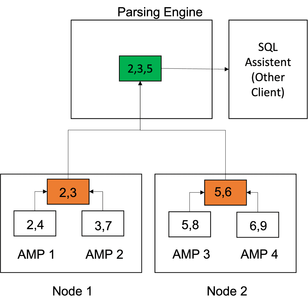
Teradata uses a sorting algorithm to arrange data in a specific order.
This sorting algorithm’s exceptional performance comes from the following qualities:
- The AMP local pre-sorting step is done in parallel on all AMPs, and sort performance increases with the system size (good scalability).
- Teradata must sort only the client-requested rows in the last global merge step. Usually, when the client requests the whole table (such as in SQL Assistant), we cancel the request after having a small number of rows on our screen. It would not make sense to perform the global sort for millions of rows that the user will never see.
Partial Redistribution and Duplication
Introduction to Teradata Partial Redistribution and Partial Duplication
Managing data skew is a critical aspect of optimizing Teradata performance. While table-level skew can typically be prevented by selecting an appropriate Primary Index, spool skew occurs during query execution – a common and often significant problem.
Spool skew is a common issue when joining tables in Teradata. The join process is executed simultaneously by all available AMPs in parallel.
Let us consider the following example of a join:
B … Big table with 100 Million rows
S … Small table with 10,000 rows
Assuming that the two tables are joined on a column that is not the primary index for either table, the optimizer may rehash and redistribute both tables. This approach is ideal if the join column values are evenly distributed across all AMPs.
We assume that in the big table B, the value in the join column is the same for approximately 99% of the rows. This equates to 99 million out of 100 million rows sharing the same value in the join column.
Currently, we are experiencing a significant performance issue due to data skew.
Rehashing the rows assigns 99 million rows to a single AMP because they share the same hash value.
The AMP designated for receiving may experience a Hot AMP situation and deplete its spool space.
Before Teradata Release 13, a performance specialist’s sole responsibility was to address dynamic skew issues by manipulating the optimizer to adopt an alternate execution plan. This issue could occasionally be resolved by incorporating statistics, while in other cases, the only viable solution was to rewrite the SQL statement fully.
Teradata 14 introduced a refined approach to resolve data skew problems.
The AMP is informed of any skewed values pertaining to the big Table B.
Skewed rows in Table B remain confined to their respective AMPs. Non-skewed rows are redistributed by rehashing the join column(s).
Non-biased rows from small table S are rehashed on their join column(s), while rows that would become skewed during redistribution are duplicated across all AMPs.
Upon completing the partial redistribution and duplication of the tables, each AMP proceeds to generate the initial result by merging the contents of the redistributed spools.
Each AMP produces a secondary output by merging table S’s replicated spool contents with table B’s local spool.
With Teradata 14, PRPD alleviates certain performance issues related to skew. However, the Teradata optimizer requires knowledge of biased values, underscoring the importance of maintaining up-to-date statistics.
Partial GROUP BY
What is Partial Group By?
Joins are costly. Before the introduction of PARTIAL GROUP BY, the join would be performed first, and then the aggregated result would follow.
PARTIAL GROUP BY reduces the amount of data that must be redistributed or duplicated to all AMPs during join preparation by performing aggregations before the join, without altering the query’s semantics.
The savings increase as the number of unique values in the GROUP BY columns decreases.
Early GROUP BY and Partial GROUP BY are distinguishable solely based on their approach to aggregations in relation to the join process. While Early GROUP BY executes all aggregations before joining, Partial GROUP BY conducts a portion of the aggregation before and after the join. Nonetheless, this is the only point of differentiation.
This query is optimized for PARTIAL GROUP BY:
SELECT table1.key,SUM(table1.fact),SUM(table2.fact)

FROM table1 INNER JOIN table2 ON table1.key = table2.key

GROUP BY 1;
The order of the join and aggregation is irrelevant in this scenario. The performance may vary based on the number of rows and distinct values in the “fact” column of each table.
Reducing the Resource Cost of Joins
Joining tables can be costly since each join requires that the rows being joined are on the same AMP. In cases where the two tables possess different primary indices, copying one or both tables’ rows may be necessary, which can cause a high number of I/Os in large tables. The Teradata Optimizer can select from various join methods for each join, tailored for a specific scenario. The primary objective of the Teradata Optimizer is to minimize resource consumption, including I/Os, CPU seconds, network traffic, and other factors, for the entire execution plan.
General Teradata Join Optimization Considerations
The optimizer utilizes statistics to determine the optimal join plan and estimates the cost of each join based on the following factors:
- The expected cardinality of the output spool (after the join) and
- The expected cardinality of the input spools after WHERE conditions have been applied.
- The selected column lists each input spool and the average row size. Usually, only the selected columns of each input spool are taken over into the resulting spool.
The only exception is if a permanent table is joined directly without spooling. In such a case, all columns of this table are copied into the resulting spool.
Based on the above observations, we can draw the following conclusions regarding performance:
The essential statistics for each join are the ones on the join columns and any available WHERE condition.
We should apply WHERE conditions in our queries whenever possible to reduce the input tables’ cardinality.
Further, we should only select the columns required in the result set and avoid „SELECT * FROM“ queries.
Tuning with the PERIOD Data Type
This article presents a case study from my previous projects. Specifically, it showcases an implementation that generates rows for all days between a start date and an end date based on a primary key. To illustrate the issue, I have simplified the query. The following example serves as a demonstration:
| Primary Key | Start Date | End Date |
| 1 | 2022-09-12 | 2022-09-15 |
| Primary Key | Start Date | End Date | Calculated Date |
| 1 | 2022-09-12 | 2022-09-15 | 2022-09-12 |
| 1 | 2022-09-12 | 2022-09-15 | 2022-09-13 |
| 1 | 2022-09-12 | 2022-09-15 | 2022-09-14 |
| 1 | 2022-09-12 | 2022-09-15 | 2022-09-15 |
Here is the implementation I optimized. Initially, the problem was resolved using a recursive query, which performed well. However, as the data expanded significantly, the query’s runtime increased substantially.
SET QUERY_BAND = ‘DWHPRO=RECURSION;’ FOR SESSION;
SELECT PK, START_DATE, END_DATE, CALC_DATE
FROM (
WITH RECURSIVE RecTable (PK,START_DATE,END_DATE,CALC_DATE) AS
(SELECT t01.PK,t01.START_DATE, DATE AS END_DATE, START_DATE AS CALC_DATE
FROM PERFTEST t01
WHERE START_DATE BETWEEN DATE’1900-01-01′ AND DATE+1UNION ALL
SELECT PK,START_DATE,END_DATE,CALC_DATE + INTERVAL ‘1’ DAY AS CALC_DATE
FROM RecTable
WHERE (CALC_DATE < END_DATE )
)
SELECT * FROM RecTable
) A
ORDER BY PK, CALC_DATE;
| QueryBand | TotalIOCount | AMPCPUTime | SpoolUsage | StartTime | FirstRespTime |
| RECURSION | 700180812,00 | 38859,82 | 348420681728 | 13.09.2022 19:11:11.830000 | 13.09.2022 19:17:28.820000 |
Below you can see the optimized query:
SET QUERY_BAND = ‘DWH=EXPAND;’ FOR SESSION;
SELECT PK, START_DT, DATE AS END_DT, BEGIN(CC) AS CALC_DATE
FROM PERFTEST T01
WHERE START_DT BETWEEN DATE’1900-01-01′ AND DATE
EXPAND ON PERIOD(START_DT,DATE+1) AS CC BY INTERVAL ‘1’ DAY
ORDER BY PK,CALC_DATE
| QueryBand | TotalIOCount | AMPCPUTime | SpoolUsage | StartTime | FirstRespTime |
| EXPAND | 7084187,00 | 11141,82 | 348420681728 | 13.09.2022 19:19:23.120000 | 13.09.2022 19:19:41.360000 |
The improved query requires 99% fewer IO operations than the initial query and 71% fewer CPU seconds. Spool utilization has remained constant.
The case study highlighted Teradata’s potential for significant performance improvements through query optimization. Rewriting the SQL itself can often yield greater efficiency without relying on optimizer hints.
Comparison Operators and Performance
The performance of Teradata is somewhat dependent on its comparison operators.
Selecting the appropriate comparison operator is crucial in distinguishing between efficient and inefficient queries.
How do the chosen comparison operators affect performance?
Quality statistics are a crucial input for the Teradata Optimizer, significantly influencing the execution plan’s aggressiveness or conservatism.
Teradata stores column-level statistics, which can be used for substrings of a column despite the inability to collect statistics at a finer granularity. Teradata 14.10 offers expanded capabilities for utilizing available statistics compared to previous versions.
Consider a SQL query featuring a WHERE clause targeting a designated column. Supposing a code is stored in a character column titled “ORIGIN_CD,” our objective is to gather all entries where the column begins with the letter ‘A.’
There are various ways to execute this SQL statement, and each option may yield a unique execution plan with distinct access paths, runtimes, and resource usage patterns.
SELECT * FROM <TABLE> WHERE ORIGIN_CD LIKE ‘A%’;
SELECT * FROM <TABLE> WHERE SUBSTR(ORIGIN_CD,1,1) = ‘A’;
In both cases, applying a function to the “ORIGIN_CD” column may hinder the Optimizer from utilizing column statistics, depending on your Teradata version. Avoiding functions on columns present in a WHERE or JOIN condition is recommended. Using functions on join columns could indicate a poor design or an outdated data model.
Conclusion:
Explore alternative solutions to enhance performance when applying functions to WHERE and JOIN conditions.
Generating Number Ranges Without a Table
Method 1, avoiding any helper tables or functions which are only available in new releases of Teradata:
WITH RECURSIVE NumberRanges(TheNumber,TheString) AS
(
SELECT 1 AS TheNumber,casT(1 as VARCHAR(500)) as TheString

FROM
(
  SELECT * FROM (SELECT NULL AS X) X
) DUMMYTABLE
UNION ALL
SELECT
	TheNumber + 1 AS TheNumber,
	TheString ||',' || TRIM(TheNumber+1)

FROM NumberRanges
WHERE
TheNumber < 10
)
SELECT TheString
FROM NumberRanges
QUALIFY ROW_NUMBER() OVER ( ORDER BY TheNumber DESC) = 1
Method 2, with helper tables and XMLAGG:
SELECT
     TRIM(TRAILING ',' FROM (XMLAGG(TRIM(rn)|| ',' ) (VARCHAR(255))))
 FROM
     (SELECT 1 + ROW_NUMBER() OVER (ORDER BY Sys_Calendar."CALENDAR".day_of_calendar) as rn
 FROM Sys_Calendar."CALENDAR" QUALIFY rn <= 10) t;
Both methods deliver the string “1,2,3,4,5,6,7,8,9,10”.
Which process do you believe is using fewer Disk IOs and CPU resources?
Several individual rewrites have their own walkthroughs: when UNION ALL beats UNION, what GROUP BY costs in Teradata, IN against BETWEEN, and why the plans differ, the join methods relational engines choose between and the cursor mistakes that quietly serialise a procedure.
More rewrites, each worked through separately: replacing an update-then-insert pair with MERGE, the five decisions behind every window aggregate, combining sets without paying for UNION, where DECIMAL arithmetic stops adding up and diagnosing a LIKE that will not use an index.
Three further SQL constructs worth knowing: selecting every column except a few, the ordered analytical functions and what they cost and GROUPING SETS, ROLLUP and CUBE.
Related Services
⚡ Need Help Optimizing Your Data Platform?
We cut data platform costs by 30–60% without hardware changes. 25+ years of hands-on tuning experience.
Explore Our Services →📋 Considering a Move From Teradata?
Get a personalized migration roadmap in 2 minutes. We have migrated billions of rows from Teradata to Snowflake, Databricks, and more.
Free Migration Assessment →