
In the past, Teradata and similar databases used a logical row format to store data. This was beneficial for the main functions of these databases, such as handling transactions and conducting queries. The data was effectively organized on the disks by keeping the columns of a record together in the same data blocks.
Different index types are available to improve row retrieval speed. While B+ trees are commonly utilized in many relational databases for index storage, Teradata employs a hashing algorithm for table row lookups. One exception is the non-unique secondary index, which follows a distinct design.
Row-based data layout facilitates swift data access for small data sets, enabling the coexistence of OLTP and strategic queries. Indexing can expedite data retrieval.
In the era of Big Data, Teradata stores an exponentially growing number of rows and columns.
Queries typically require only a few columns, but unfortunately, all columns must still be retrieved.
The number of I/Os necessary for data retrieval rises as the data rows expand in width. This results in less efficient query processing from both performance and storage standpoints. Teradata must transfer the entire row from the disk to the AMP’s FSG cache, even if just one column is being accessed.
Column-oriented databases offer a distinct method of arranging data on disks and have been introduced as an alternative. Teradata 14.00 includes this feature by incorporating columnar storage.
Column-partitioned tables are not universally NoPI: documented configurations include PI, PA and NoPI, with release-specific restrictions. The NoPI definitions below are examples of one design choice.
Columnar databases store columns or column sets in data blocks rather than rows. The columns of a single row are randomly dispersed across separate data blocks.
Columnar Databases Store Columns or Column Sets
A single AMP manages related columns, while each AMP retains the entirety of a row’s data through vertical partitioning.
The following example illustrates the difference between row and columnar storage:
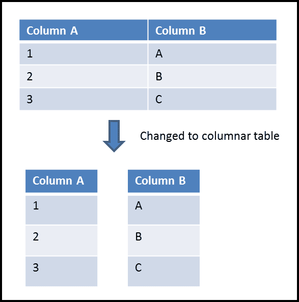
All containers maintain the same number of rows in the identical order, i.e., the relative row number. If a query solely selects “Column A,” it will only require moving this single column to the AMP’s FSG cache.

Get the complete Teradata tuning book, free
Teradata Query Performance Tuning: The DWHPro Guide
By Roland Wenzlofsky & Artemios Vogiatzis
206 pages on statistics and demographics, access paths and indexes, query execution plans, and joins. Get the full PDF and practical Teradata updates from DWHPro.
Confirm your email to receive your download link. Privacy policy. Unsubscribe in any newsletter.
About the free book“How does record retrieval work for a query such as the one mentioned above?”
SELECT COLUMN_A FROM THE_TABLE WHERE COLUMN_B = 'C';To retrieve the associated value for COLUMN_A, it is necessary to transfer both column stores, COLUMN_A and COLUMN_B, to the FSG cache. By utilizing the precise sequence of data within the containers, COLUMN_A’s value can be obtained by referencing its corresponding row number, which in this case is 3.
The following historical DDL illustrates column partitioning. Column partitioning was unavailable in the audit system, so these definitions were not runtime-verified; validate them on a system supporting the feature.
CREATE TABLE the_table
(
 PK INTEGER,

COLUMN_A CHAR(01),

COLUMN_B CHAR(01)

) NO PRIMARY INDEX

PARTITION BY COLUMN;
To create a multicolumn container, utilize the following syntax to create one container for each column.
Multicolumn Container Syntax
CREATE TABLE the_table
(

PK INTEGER,

COLUMN_A CHAR(01),

COLUMN_B CHAR(01)

) NO PRIMARY INDEX

PARTITION BY COLUMN (PK, (COLUMN_A,COLUMN_B))

;
The primary key (PK) will be stored in a singular container, while columns COLUMN_A and COLUMN_B will reside together in a separate, multi-column container.
Teradata employs two distinct physical column store designs wherein columns are stored in containers, i.e. physical rows containing one or multiple table columns. These containers hold an equal number of rows, each containing a relative row number that facilitates grouping columns from the same data row.
Teradata allows the creation of either single-column or multicolumn containers. In addition, Teradata supports mixed storage of these formats.
Column sets can be stored like traditional rows, with the remaining columns stored in containers. Teradata autonomously determines the optimal storage format when column storage is utilized. This hybrid storage approach can be implemented with the following statement:
CREATE TABLE YourTable
(PK INTEGER, COLUMN_1 INTEGER, COLUMN_2 INTEGER)
NO PRIMARY INDEX
PARTITION BY COLUMN (COLUMN_1, ROW(PK,COLUMN_2));
Mixed configurations are applicable in certain circumstances. For instance, COLUMN_1 may possess high compressibility, whereas PK and COLUMN_2 commonly feature in queries.
A container is a data block comprising a subset of columns from multiple rows. If a single container cannot accommodate all the column values of each row, additional containers are dynamically generated.
Columnar data storage proves useful in OLAP for quick access to vast amounts of data where only a handful of columns are relevant to the desired result set, such as the summation of all customer balances.
A NoPI column-partitioned table has no PI hash access, but this is not a universal restriction of column partitioning. Available access paths depend on the table definition and release.
Access Paths for NoPI Column-Partitioned Tables
To include information on “all customers” in OLAP, indexing data using the Teradata hashing algorithm does not enhance performance. This is because direct access indexing techniques are ineffective for retrieving all rows.
Improving performance relies on accessing fewer data blocks, specifically those that contain the desired columns.
Teradata handles both row and column orientation well. However, the developer must assess which design to implement and when. This decision involves several factors, as each type of storage — whether row or column-oriented — has its own set of benefits and drawbacks.
The primary drawback of implementing Teradata’s column storage is that it complicates joins, requiring the conversion of columns from various containers into rows.
Updates and deletes can create additional storage and maintenance work in column partitions. The amount depends on affected data, representation and reclamation; updating rows does not universally double table space.
Teradata can efficiently compress column containers without the need for explicit instructions to the system. Compression is particularly effective for single-column containers.
Although row-level compression is often restricted due to the typically high cardinality of data tuples, columnar compression is more feasible as columns may only contain a small number of distinct values, such as the code columns “male” and “female”. By utilizing dictionary compression, which has been available in Teradata since the implementation of single-value compression and MVC, the column values of all rows can be compressed into just a few bits.
However, Teradata’s implementation of column storage is not state-of-the-art as it retrieves and reconstructs rows by decompressing data from column containers. The traditional row-based database engine then operates on the already decompressed data.
Compression Recommendations for Column-Stored Tables
It is advisable to consider multi-value and block-level compression for column-stored tables.
This method is not as I/O intensive as Oracle’s Exadata approach, which involves storing mini-column collections within data blocks that are solely associated with the corresponding data block rows. Nevertheless, more capable alternatives exist that do not rely on conventional row-focused engines, such as SAP HANA and Vertica.
Note that the aforementioned factors pertain to a workload that is optimal for column stores. This does not indicate that Oracle’s implementation is consistently inferior to Teradata’s implementation or vice versa. The nature of the workload is the determining factor.
Teradata’s columnar feature can be accessed in Version 14.00.
Create a columnar table in Teradata with the following example:
CREATE TABLE the_table

(

PK INTEGER,

ATTRIB CHAR(10)
) NO PRIMARY INDEX
PARTITION BY COLUMN;
A query like “SELECT ATTRIB FROM <TABLE>” would only require moving column ATTRIB into the AMP’s FSG memory.
Loading support depends on the utility, table definition and release. A staging NoPI table followed by INSERT … SELECT is one possible design, not a universally optimal or mandatory path.
Both column storage and row-level partitioning can coexist within a table using this syntax:
CREATE TABLE the_table
(PK INTEGER, MY_DATE DATE)
NO PRIMARY INDEX
PARTITION BY (COLUMN, RANGE_N(MY_DATE BETWEEN DATE '2014-01-01'
AND DATE '2014-12-31' EACH INTERVAL '1' DAY));Deciding what to change in your data platform?
Compare optimisation, modernisation and migration against your workload and business requirements.
Get the complete Teradata tuning book, free
Teradata Query Performance Tuning: The DWHPro Guide
By Roland Wenzlofsky & Artemios Vogiatzis
206 pages on statistics and demographics, access paths and indexes, query execution plans, and joins. Get the full PDF and practical Teradata updates from DWHPro.
Confirm your email to receive your download link. Privacy policy. Unsubscribe in any newsletter.
About the free book
Deleted records are marked as deleted but not removed from the disk. What is the logic behind that?
@MALIK HASSAN QAYYUM
Performance would be really bad
Nice article.Clearly explained.
Thanks