Teradata Heuristics are utilized in cases where statistics for a non-indexed column are unavailable. They serve as rules of thumb for approximating the number of selected data rows and are employed in WHERE condition predicates and join planning.
What is Teradata Heuristics?
Teradata Heuristics estimate a percentage of table cardinality to determine the number of selected data rows. You may question how the optimizer obtains the table cardinality.
The optimizer can estimate table cardinality using collected summary or primary index statistics. Without statistics, the optimizer can still obtain a random AMP sample for the same purpose.
Teradata Optimizer’s estimations rely solely on table cardinality. In this post, we will examine multiple queries and their heuristic estimates. Additionally, we will explore superior methods to replace heuristic estimations with more precise alternatives. It is crucial to avoid relying on heuristic estimates as they may provide flawed statistical information to the Teradata Optimizer.
Teradata Heuristics and non-indexed Columns
Nonindexed column statistics are crucial for WHERE condition predicates. We will begin with simple examples to explain basic heuristic concepts and subsequently introduce more intricate configurations.
Before delving into the specifics of heuristics, an essential point to note:
Note that the information provided pertains specifically to nonindexed columns. When discussing the number of selected rows or the percentage of selected rows, the estimation of table rows is based on either collected summary or index statistics or a random AMP sample. It’s important to remember that when we refer to table row counts, we are referring to estimates rather than actual figures.
Examples of Heuristics Usage
We refer to estimations rather than the actual row numbers when discussing table row counts. The subsequent test table, utilized in all examples, has a row count of 100,000 and is the foundation for the optimizer’s heuristic estimations.
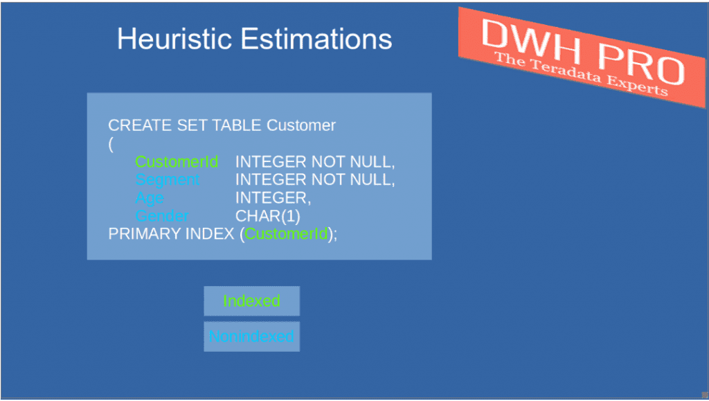
We will start our tour with a very simple example, having only one WHERE condition predicate for a nonindexed column (” segment” is neither the primary index nor any other index of the customer table)
Here is our test query: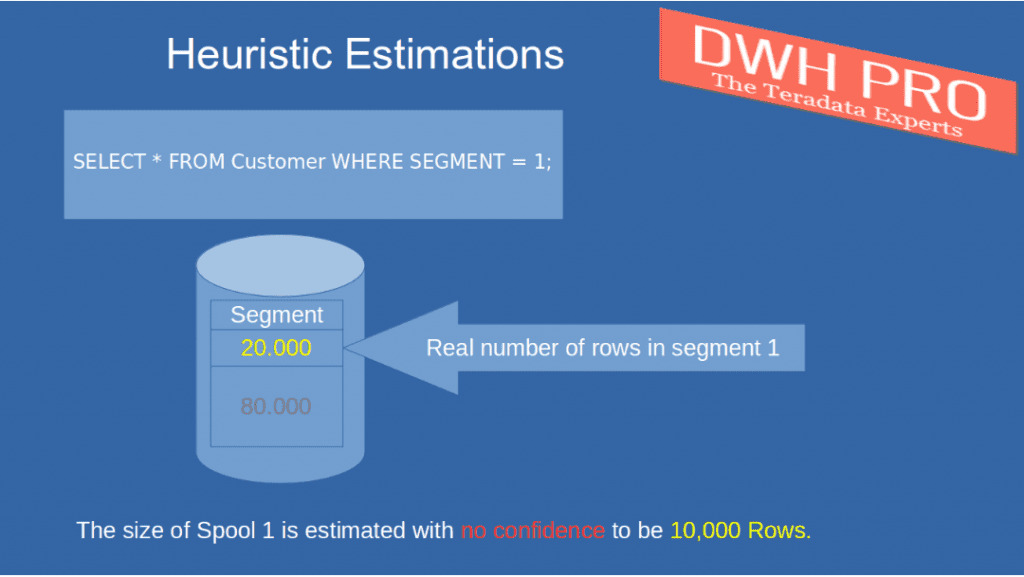
We gathered data on the main index column of the “customer” table. Based on these statistics, the estimated number of rows is 100,000.
No statistics were gathered for the unindexed “segment” column.
The actual number of rows in “Segment 1” is 20.000.
The optimizer utilizes Teradata heuristics to estimate values for the “segment” column, which is not indexed.
The number of selected rows is estimated to be 10% of the table rows.
The inflexible rule is a non-negotiable 10% with no exemptions.
100.000 * 10% = 10.000 rows
The optimizer miscalculated the data rows by 50%, underestimating the actual count. Even if segment 1 had no rows, the estimation would remain 10,000, significantly overestimating selected rows.
The “10% Rule” is the optimizer’s baseline estimate when there is only one WHERE condition predicate for a single value. An example demonstrates why heuristic estimates should be avoided, as they frequently diverge from reality.
In this example, we will include another WHERE condition for a second non-indexed column in the query.
We did not gather statistics on the columns utilized in the predicates. Here is our test inquiry:
SELECT * FROM Customer WHERE SEGMENT = 1 AND Age = 25;
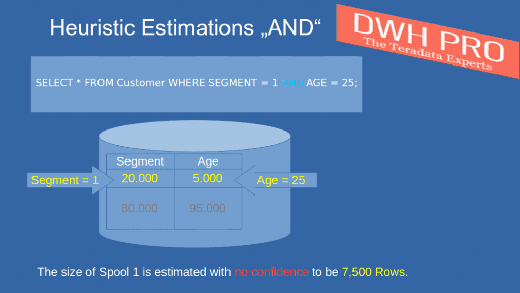
The Teradata heuristics rule applied for nonindexed columns which are AND combined is:
We increase the initial estimate by 75% for each combined AND predicate.
Let’s estimate our example query.
10% from 100.000 data rows = 10.000 rows. This is the base estimation. We multiply the base estimation by 75%, i.e., 10.000 * 75%. The result is 7.500 rows.
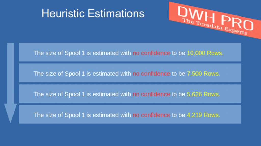
Adding another WHERE condition predicate would result in the following total estimate for our example:
((100.000 * 10%) *75%) * 75% = 5.625 data rows.
Adding one more WHERE condition predicate would reduce the rows to 4,219.
Adding more WHERE conditions with “AND” reduces the estimated number of rows:
In this example, we will explore the implementation of heuristic estimates for WHERE condition predicates on OR combined columns.
SELECT * FROM Customer WHERE SEGMENT = 1 OR Age = 25;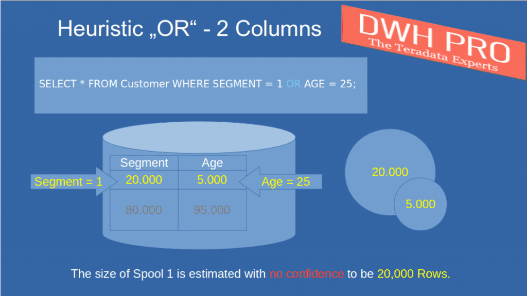
The guideline for OR predicates that are combined across multiple columns is as follows:
The predicate estimate is based on our original estimation of 10% of the total rows in the table.
The customer table is estimated to contain 100,000 rows.
The estimation for the result set of the query is (100.000 * 10%) + (100.000 * 10%), or 20.000 rows (2 times the base estimation)
As with the prior example, approximations will either exceed or fall short and are unlikely to align with the chosen row count.
Naturally, there is a limit to the estimation. Combining 11 conditions with “OR” will not yield an estimate of 110%, but rather 100%.
These heuristic rules provide valuable insight and aid in understanding execution plan estimations. The estimation process for OR combined predicates on identical columns is more intricate.
We deciphered the algorithm and extracted the fundamental principles and components.
The optimizer differentiates between ranges and single values.
We will begin with estimating single-value predicates.
SELECT * FROM Customer WHERE Age in (20,22,24);
SELECT * FROM Customer WHERE Age = 20 OR AGE = 22 OR Age = 24;
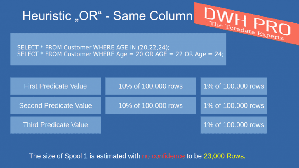
The optimizer assumes that only the first two predicates will select 10% of the table rows.
From the second predicate onwards, all predicates, including the first one, will add 1% of the table’s cardinality. However, from the third predicate onwards, there will be no base estimation, which is typically 10% of the table’s cardinality. In our example, this translates to:
(100.000 * 10%) for the first predicate
(100.000 * 10%) for the second predicate
(3 * (100.000 * 1%)) = 3.000 for the three predicates.
The total estimation, therefore, is 23.000 rows.
Estimations for Ranges of Values
Examples of range predicates with contiguous selected values.
SELECT * FROM Customer WHERE Age in (20,21,22);
SELECT * FROM Customer WHERE Age BETWEEN 20 AND 22;
SELECT * FROM Customer WHERE Age = 20 OR AGE = 21 OR Age = 22;

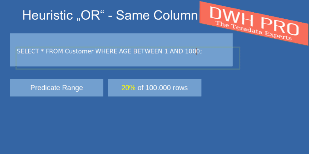
When our WHERE condition features a single range predicate, the estimation will be 20% of the table’s total rows. In this particular example, the estimated number of rows is 20,000.
The number of values within the ranges is inconsequential. This query will yield an estimation of 20% regardless.
SELECT * FROM Customer WHERE Age BETWEEN 1 AND 1000;
Including a second range in our query would increase the estimation to 40%, which is double the initial 20%.
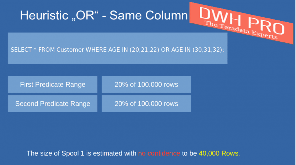
If we introduce a third range, a more precise estimation is utilized. The assessment for the first and second range criteria is 10% each, whereas, in the previous example with two ranges, it was 20% per range criterion.
No additional 10% estimations will be added beyond the second range predicate. However, akin to estimations for individual values, the count of unique values within the range is tallied, and the estimate is augmented by 1% per value.
SELECT * FROM Customer WHERE Age IN (10,11,12) OR AGE IN (20,21,22) OR AGE IN (30,31,32);
For instance, this implies:
(100.000 * 10%) for the first range predicate
(100.000 * 10%) for the second range predicate
(9 * (100.000 * 1%)) = 9.000 for the nine values.
The total estimation, therefore, is 29.000 rows.
The estimated percentage for a single range predicate is consistently 20%, and the quantity of unique range values does not affect this estimation.
The estimation for dual range predicates rises to 40%, regardless of the number of unique range values.
If our query has three or more range predicates, the estimation for the first two ranges is 20% (10% plus 10%), and each distinct value of all ranges increases the estimate by 1%.
We will now ask: “What is the impact on heuristic estimations if we collect statistics on one or more of the WHERE condition predicates”?
The optimizer evaluates all WHERE conditions using gathered statistics and selects the estimation with the greatest selectivity as the initial point for further estimations.
The estimations will not begin with the traditional heuristic estimation of 10%, 20%, etc. Rather, they will commence with a superior estimate derived from gathered statistics. To illustrate:
Initially, we choose statistics from the CustomerAge column.
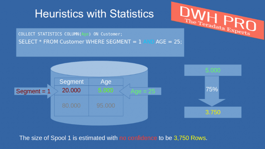
COLLECT STATISTICS COLUMN(Age) ON Customer;
We estimate 5,000 data rows for customers aged 25.
We execute the SELECT statement.
SELECT * FROM Customer WHERE Segment = 1 AND Age = 25;
The columns are unindexed.
Our estimations will commence with the data collected from a single column consisting of 5,000 rows that exhibit selectivity for CustomerAge=25.
Similar to the previous example involving combined AND conditions, the optimizer will utilize heuristics for the second column.
5.000 * 75% = 3.750 data rows.
The presence of a single column of collected statistics can significantly improve the accuracy of the estimation. As an illustration, consider the combination of three columns using the logical operator “AND,” of which two contain collected statistics while one does not.
All columns are non-indexed, which should be evident.
We gather data in two columns.
COLLECT STATISTICS COLUMN(CustomerAge) ON Customer;
COLLECT STATISTICS COLUMN(Gender) ON Customer;
There are 5,000 rows of customer age data collected, while only 100 rows have an unknown value for gender (designated as ‘U’).
Like the previous instance, the optimizer selects the column with the greatest selectivity as its preliminary approximation. In this case, that value is 100 rows.
The collected statistics in the second column are irrelevant to the optimizer. The estimations in both the second and third columns are calculated using the same 75% rule mentioned previously.
(100 * 75%) * 75% = 56.25 rows (which will be rounded to 57 rows).
SELECT * FROM Customer WHERE CustomerId = 1 AND CustomerAge = 25 AND Gender=’U’;
This final example showcases a fusion of “OR” merged columns with and without statistics (apologies for the lack of visual aid).
We collect statistics on customer age:
COLLECT STATISTICS COLUMN(CustomerAge) ON Customer;
SELECT * FROM Customer WHERE CustomerId = 1 OR CustomerAge = 25;
The optimizer calculates estimates by adding collected statistics and heuristic estimates for columns lacking statistics.
Again, the estimation for CustomerAge=25 is 5.000 rows. Heuristics for CustomerId=1 give 10.000 rows (100.000 * 10%).
The estimate is 15,000 rows.
Numerous heuristic estimation instances exist for WHERE condition predicates. However, we will conclude with a few final examples of commonly used ones.
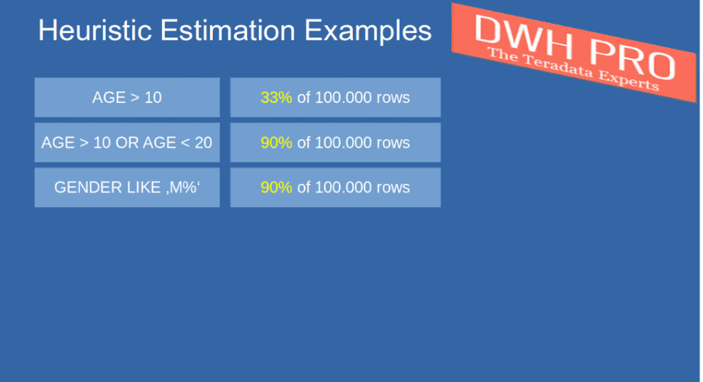

These are without collected statistics on AGE and GENDER
Great article and examples.
I’ve got a question regarding the last frequently used WHERE conditions predicate example. Are these heuristic estimates based on a table which has no collected statistics on AGE and GENDER columns?