Introduction
Teradata offers several methods for conducting joins, but all necessitate one prerequisite.
The paired table rows must reside on identical AMPs.
The chosen method for joining and relocating data is called a join strategy.
The preparation for each join method varies. The choice of Teradata join strategy utilized by the Optimizer is determined by the cost evaluation of each strategy.
Cost factors for Teradata include number of table rows, required data copying, and sorting. The Optimizer relies on accurate statistics to properly capture data demographics.
How Teradata Optimizes the Join Operations
Teradata minimizes spool usage by employing efficient join techniques that reduce the amount of copied data.
- Copy only the columns required by the request
- Apply the WHERE conditions before copying rows to a common AMP
- Whenever possible, spool the smaller table
Here is a basic illustration of calculating the necessary spool.
Table “Customer” has 1000 rows, each needing 100 bytes.
Table “Sale” has 10000 rows, each needing 500 bytes.
SELECT t01.*,t02.SalesId
FROM Customer t01 INNER JOIN Sales t02
ON t01.CustomerId = t02.CustomerId;
Selecting all columns of the “Customer” table requires 100,000 bytes of spool space (1000 x 100).
We select only the “SalesId” column from the “Sales” table, assuming it is an 8-byte INTEGER data type, which would require 80,000 bytes of spool space.
The Optimizer uses the calculated spool space to determine the distribution of tables to a common AMP.
How You Can Optimize the Join Operations
- Collect statistics on all joined columns
- Don’t apply functions on the join columns
- Always do equality joins to avoid a product join
This article will explore frequently employed join techniques and their associated strategies.
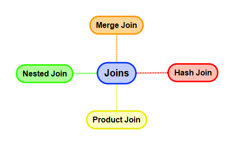
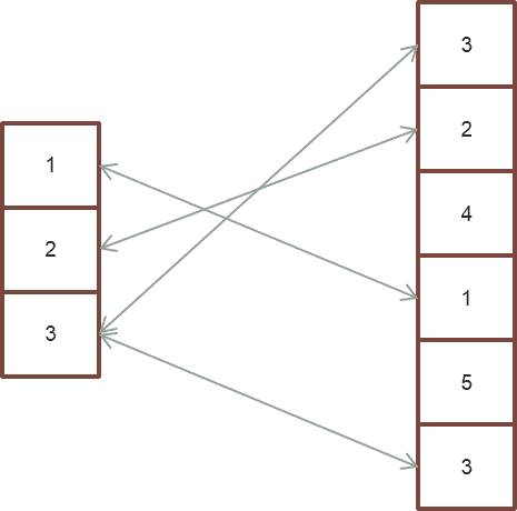
1. Teradata Merge Join – The Swiss Army Knife
When will it be used?
- The Optimizer can only use it for equality joins
Preconditions
- The rows to be joined have to be on a common AMP
- Teradata needs to sort both spools by the row hash calculated over the join column(s)
Merge Joins Algorithms
Operation
Slow Path (The Optimizer uses an index on the left table)
- The ROWHASH of each qualifying row in the left spool is used to lookup matching rows with identical ROWHASH in the right spool (using a binary search as both spools are sorted by row hash)
Fast Path (The Optimizer uses no index)
- No Index is used. The tables are fully scanned, alternating from the left to the right side; the row hash match is done.
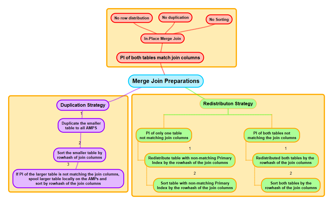
The Non-PPI Merge Join Strategies
Possible Join Preparation
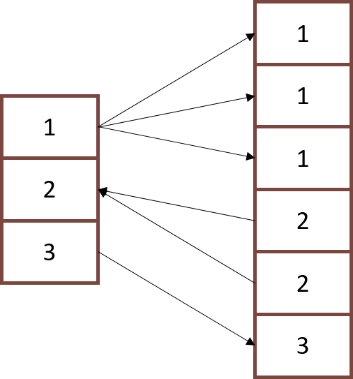
- Re-Distribution of one or both spools by ROWHASH or
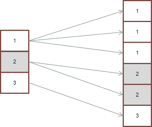
- Duplication of the smaller spool to all AMPs
- Sorting of one or both spools by the ROWID
The join columns define the common AMP of rows from two spools the Optimizer wants to join. This leaves us with 4 data distribution scenarios:
- The Primary Indexes (or any other suitable index) of both tables equal the join columns: No join preparation is needed as the rows to be joined are already on the common AMP and sorted by the row hash.
Hint: The Primary Index of both tables needs to include all join columns, but it can have additional columns. These are applied as residual conditions. It’s only crucial that - Only one table’s primary index (or any other suitable index) matches the join columns: The second table’s rows must be relocated to the common AMP.
- Neither the Primary Index of the first table (or any other suitable index) nor the Primary Index (or any other appropriate index) of the second table matches the joined columns: The rows of both tables must be relocated to the common AMP.
To relocate rows to the shared AMP, you can redistribute them using the ROWHASH join column(s), or duplicate the smaller table across all AMPs.
If the Optimizer chooses to replicate the smaller table to all AMPs, it will then be sorted in the subsequent step by computing the rowhash of the joined columns and arranging them in order.
If the primary index does not match the joined columns, the bigger table must also undergo hashing and sorting. Subsequently, the bigger table is spooled locally to the AMP.
Performance Considerations
This join’s efficiency relies on identical primary indexes in both tables, which eliminates the need for Teradata to transfer any rows between AMPs.
The join method is highly robust in various aspects, as any performance loss is limited. This occurs in cases where the optimizer has underestimated the number of rows in tables due to incorrect or missing statistics.
Additionally, as both tables are sorted by rowhash, Teradata only needs to copy each data block into the main memory once, providing an extra benefit.
The PPI Merge Join Strategies
The Optimizer can utilize all methods, even when joining involves PPI tables.
If a non-partitioned table is joined with a PPI table, the Optimizer can transform the PPI table into a non-partitioned table and apply one of the strategies.
The Optimizer can partition a non-partitioned table like a PPI table when joining with an un-partitioned table.
This is only feasible if the non-partitioned table contains all partition columns.
The Optimizer can utilize unique merge join methods if there is one partitioned table.
- Rowkey-Based Merge Join
- Single Window Merge Join
- Sliding Window Merge Join
The Rowkey-Based Merge Join
The Rowkey-Based Merge Join can be direct; neither of the two tables involved is spooled.
To perform a rowkey-based merge join, it is necessary for the tables to share identical primary indices and partitioning. Additionally, the join must be an equijoin conducted through the primary index and partition columns.
If these requirements are not met, the Optimizer may still opt for a merge join based on the rowkey, but it will require preparation for the join rather than a direct join.
In a PPI table join with an unpartitioned table, the optimizer can rearrange the unpartitioned table to match the primary index and partitions of the PPI table to execute a rowkey-based merge join.
The Rowkey-Based Merge Join and CHARACTER SETS
When joining two PPI tables that use Character Partitioning, it is essential to ensure that the CHARACTER SET of the partition columns is identical. Otherwise, the Rowkey-Based Merge Join cannot be direct, but the table with CHARACTER SET LATIN must first be spooled to make the row keys of both tables identical.
Here is an example. Both tables are identical, except for the CHARACTER SET of Column PartCol1.
Explain SELECT *
FROM MergeJoinChar1 t01
INNER JOIN
MergeJoinChar2 t02
ON
t01.PK = t02.PK
AND t01.PartCol1 = t02.PartCol1;
1) First, we lock DWHPRO.t02 in TD_MAP1 for read on a reserved
RowHash in all partitions to prevent global deadlock.
2) Next, we lock DWHPRO.t01 in TD_MAP1 for read on a reserved RowHash
in all partitions to prevent global deadlock.
3) We lock DWHPRO.t02 in TD_MAP1 for read, and we lock DWHPRO.t01 in
TD_MAP1 for read.
<strong>4) We do an all-AMPs RETRIEVE step in TD_MAP1 from DWHPRO.t01 by way
of an all-rows scan with no residual conditions into Spool 2
(all_amps), which is built locally on the AMPs. Then we do a SORT
to partition Spool 2 by rowkey. The size of Spool 2 is estimated
with low confidence to be 73,420 rows (3,450,740 bytes). The
estimated time for this step is 0.29 seconds.</strong>
<strong>5) We do an all-AMPs JOIN step in TD_MAP1 from DWHPRO.t02 by way of a
RowHash match scan with no residual conditions, which is joined to
Spool 2 (Last Use) by way of a RowHash match scan. DWHPRO.t02 and
Spool 2 are joined using a rowkey-based merge join, with a join
condition of ("((TRANSLATE((PartCol1 )USING LATIN_TO_UNICODE))=
DWHPRO.t02.PartCol1) AND (PK = DWHPRO.t02.PK)"). The result goes
into Spool 1 (group_amps), which is built locally on the AMPs.
The size of Spool 1 is estimated with low confidence to be 97,878
rows (4,796,022 bytes). The estimated time for this step is 0.25
seconds.</strong>
6) Finally, we send out an END TRANSACTION step to all AMPs involved
in processing the request.
-> The contents of Spool 1 are sent back to the user as the result of
statement 1. The total estimated time is 0.53 seconds.CREATE MULTISET TABLE MergeJoinChar2
(
PK INTEGER NOT NULL,
PartCol1 CHAR(10) CHARACTER SET LATIN
) PRIMARY INDEX (PK)
PARTITION BY RANGE_N(PartCol1 BETWEEN 'A','B','C','D' AND 'Z')
;
CREATE MULTISET TABLE MergeJoinChar2
(
PK INTEGER NOT NULL,
PartCol1 CHAR(10) CHARACTER SET UNICODE
) PRIMARY INDEX (PK)
PARTITION BY RANGE_N(PartCol1 BETWEEN 'A','B','C','D' AND 'Z')
;An Example of a Rowkey-Based Merge Join
The join, in this instance, utilizes the Primary Index (PK) and Partition Columns (PartCol1) that are identical in both tables. Teradata executes a direct rowkey-based merge join, eliminating the need to spool tables.
Explain SELECT *
FROM MergeJoin1 t01
INNER JOIN
MergeJoin2 t02
ON
<strong>t01.PK = t02.PK
AND t01.PartCol1 = t02.PartCol1;</strong>
1) First, we lock DWHPRO.t02 in TD_MAP1 for read on a reserved
RowHash in all partitions to prevent global deadlock.
2) Next, we lock DWHPRO.t01 in TD_MAP1 for read on a reserved RowHash
in all partitions to prevent global deadlock.
3) We lock DWHPRO.t02 in TD_MAP1 for read, and we lock DWHPRO.t01 in
TD_MAP1 for read.
<strong> 4) We do an all-AMPs JOIN step in TD_MAP1 from DWHPRO.t02 by way of a
RowHash match scan with no residual conditions, which is joined to
DWHPRO.t01 by way of a RowHash match scan with no residual
conditions. DWHPRO.t02 and DWHPRO.t01 are joined using a
rowkey-based merge join, with a join condition of (
"(DWHPRO.t01.PartCol1 = DWHPRO.t02.PartCol1) AND (DWHPRO.t01.PK =
DWHPRO.t02.PK)").</strong> The result goes into Spool 1 (group_amps),
which is built locally on the AMPs. The size of Spool 1 is
estimated with low confidence to be 73,414 rows (2,716,318 bytes).
The estimated time for this step is 0.15 seconds.
5) Finally, we send out an END TRANSACTION step to all AMPs involved
in processing the request.
-> The contents of Spool 1 are sent back to the user as the result of
statement 1. The total estimated time is 0.15 seconds.An Example of changing both PPI Tables to Non-PPI Tables
The join, in this instance, is executed on the primary index, which is identical in both tables, and the partition columns are excluded from the join condition. The tables are of equivalent size.
The Optimizer modifies PPI and non-PPI tables by spooling and sorting them according to the rowhash of their primary index before executing a conventional rowhash match scan.
Explain SELECT *
FROM MergeJoin1 t01
INNER JOIN
MergeJoin2 t02
ON
<strong>t01.PK = t02.PK;</strong>
1) First, we lock DWHPRO.t02 in TD_MAP1 for read on a reserved
RowHash in all partitions to prevent global deadlock.
2) Next, we lock DWHPRO.t01 in TD_MAP1 for read on a reserved RowHash
in all partitions to prevent global deadlock.
3) We lock DWHPRO.t02 in TD_MAP1 for read, and we lock DWHPRO.t01 in
TD_MAP1 for read.
<strong> 4) We execute the following steps in parallel.</strong>
1) <strong>We do an all-AMPs RETRIEVE step in TD_MAP1 from DWHPRO.t02 by
way of an all-rows scan with no residual conditions into
Spool 2 (all_amps), which is built locally on the AMPs. Then
we do a SORT to order Spool 2 by the hash code of (
DWHPRO.t02.PK). The size of Spool 2 is estimated with high
confidence to be 73,414 rows (1,541,694 bytes). The
estimated time for this step is 0.27 seconds.</strong>
2) <strong>We do an all-AMPs RETRIEVE step in TD_MAP1 from DWHPRO.t01 by
way of an all-rows scan with no residual conditions into
Spool 3 (all_amps), which is built locally on the AMPs. Then
we do a SORT to order Spool 3 by the hash code of (
DWHPRO.t01.PK). The size of Spool 3 is estimated with high
confidence to be 73,414 rows (1,541,694 bytes). The
estimated time for this step is 0.27 seconds.</strong>
5) <strong>We do an all-AMPs JOIN step in TD_Map1 from Spool 2 (Last Use) by
way of a RowHash match scan, which is joined to Spool 3 (Last Use)
by way of a RowHash match scan. Spool 2 and Spool 3 are joined
using a merge join, with a join condition of ("PK = PK"). The
result goes into Spool 1 (group_amps), which is built locally on
the AMPs. The size of Spool 1 is estimated with low confidence to
be 73,414 rows (2,716,318 bytes). The estimated time for this
step is 0.17 seconds.</strong>
6) Finally, we send out an END TRANSACTION step to all AMPs involved
in processing the request.
-> The contents of Spool 1 are sent back to the user as the result of
statement 1. The total estimated time is 0.44 seconds.The Sliding Window Merge Join
The Sliding Window Merge Join is utilized to join a PPI table with:
- An unpartitioned table
- A PPI table that is not identically partitioned
This post provides a comprehensive explanation of the sliding window merge join.
An Example of a Teradata Sliding Window Merge Join
In this instance, the join solely employs the identical primary index in both tables. The sole contrast from the previous arrangement is that the second table’s magnitude is twice as large.
The Optimizer converts the smaller tables into a non-PPI table and performs a sliding window merge join.
Explain SELECT *
FROM MergeJoin1 t01
INNER JOIN
MergeJoin2 t02
ON
t01.PK = t02.PK;
1) First, we lock DWHPRO.t02 in TD_MAP1 for read on a reserved
RowHash in all partitions to prevent global deadlock.
2) Next, we lock DWHPRO.t01 in TD_MAP1 for read on a reserved RowHash
in all partitions to prevent global deadlock.
3) We lock DWHPRO.t02 in TD_MAP1 for read, and we lock DWHPRO.t01 in
TD_MAP1 for read.
<strong>4) We do an all-AMPs RETRIEVE step in TD_MAP1 from DWHPRO.t01 by way
of an all-rows scan with no residual conditions into Spool 2
(all_amps), which is built locally on the AMPs. Then we do a SORT
to order Spool 2 by the hash code of (DWHPRO.t01.PK). The size of
Spool 2 is estimated with high confidence to be 73,414 rows (
1,541,694 bytes). The estimated time for this step is 0.27
seconds.</strong>
<strong>5) We do an all-AMPs JOIN step in TD_Map1 from Spool 2 (Last Use) by
way of a RowHash match scan, which is joined to DWHPRO.t02 by way
of a RowHash match scan with no residual conditions. Spool 2 and
DWHPRO.t02 are joined using a sliding-window merge join, with a
join condition of ("PK = DWHPRO.t02.PK"). The result goes into
Spool 1 (group_amps), which is built locally on the AMPs. The
size of Spool 1 is estimated with low confidence to be 146,828
rows (5,432,636 bytes). The estimated time for this step is 0.78
seconds.</strong>
6) Finally, we send out an END TRANSACTION step to all AMPs involved
in processing the request.
-> The contents of Spool 1 are sent back to the user as the result of
statement 1. The total estimated time is 1.05 seconds.<strong>
</strong>This is an optimized query that utilized a sliding window merge join and achieved success.
2. Teradata Hash Join – The Sprinter, but only if executed in memory
When will it be used?
- The Optimizer can only use it for equality joins
Preconditions
- The rows to be joined have to be on a common AMP
- The smaller spool is sorted by the ROWHASH calculated over the join column(s) and kept in the FSG cache.
- The larger spool stays unsorted
Operation
- The larger spool is a full table scanned row by row
- Each ROWID from the bigger spools is searched in, the smaller spool (with a binary search)
Possible Join Preparation
- Re-Distribution of the smaller spool by ROWHASH or
- Duplication of the smaller spool to all AMPs
- Sorting of the smaller spool
Performance Considerations
Hash joins perform better than merge joins when meeting specific requirements.
3. Teradata Nested Join – The Fastest but scarce
Preconditions
- Spool 1 allows a unique ROWHASH access (a unique index is defined)
- Spool 2 allows any ROWHASH access (a unique or not unique index is defined)
- Nested joins must have equality join condition
Operation
- The qualifying row of spool one is accessed using any unique index (UPI, USI). Rarely can it be a NUPI, only if the Optimizer knows it returns one row.
- The row is relocated to the AMPs owning these rows of spool 2. A Nested Join uses a few AMPs if the index of Spool 2 is a UPI, NUPI, or USI. It used all-AMPs if the index of Spool 2 is a NUSI.
- Spool 2 is full table scanned, and each row is combined with the one row from Spool 1
Possible Join Preparation
- None
Performance Considerations
The nested join is highly efficient as it only requires one AMP, thus making it ideal for tactical workloads.
Interested in optimizing tactical workload? Keep reading here:
If you require in-depth knowledge on nested join, this article is tailored to your needs.
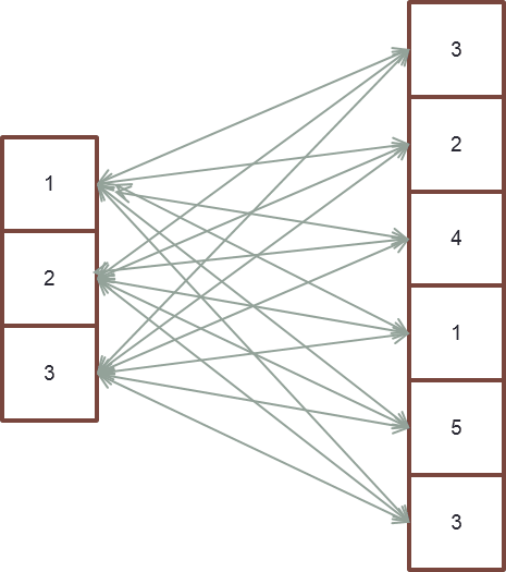
4. Teradata Product Join – The disliked Guest
When will it be used?
- The join condition is an inequality condition
- Join conditions are OR combined
- A referenced table is not used in the join condition
- The Product join is the cheapest join method
Preconditions
- The rows to be joined have to be on the AMP
- Neither of the two spools needs to be sorted
Operation
- Teradata does a full table scan on the smaller spool and
- Each qualifying row of spool one is compared with each row of spool 2
Possible Join Preparation
- Re-Distribution of one or both spools by ROWHASH or
- Duplication of the smaller spool
Performance Considerations
A product join costs are usually very high since n*m comparisons must be carried out (n = the number of rows in table1, m = number of rows in table2).
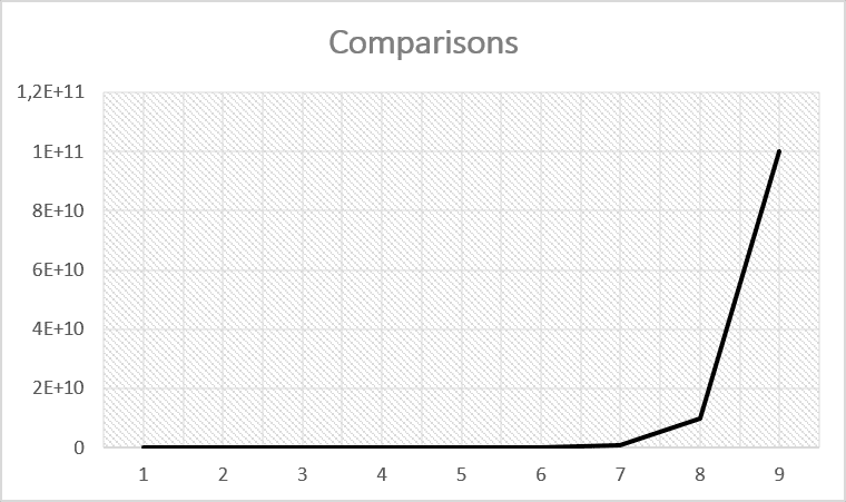
In addition to the numerous comparisons, product joins have the drawback of requiring multiple copies of data blocks from memory to main memory if Teradata cannot retain the small table completely in the main memory.

The 4 Principal Teradata Join Strategies
Hi Roland – Greetings! These concepts are useful. I would appreciate if you could please post or send me few sample queries. I am a Data Scientist/Analyst and I do not get involved at the AMP Level. This is kool. Need your help. Thank you. Regards, Sri
Hello Roland,
I like your articles. They have always described the subject very well and you provide a good parallel with real life.
I’d like to add something to the article:
1) What statement contains some inaccuracy
>> “The smaller spool is sorted by the ROWHASH calculated over the join column(s) and kept in the FSG cache”
Smaller rowset(spool is a bit incorrect term here) is not actually sorted, but a hash table is built based on hashing of smaller row set( of some part of a smaller row set if the hash table does not fit in memory).
2) >> The bigger spool is full table scanned row by row
Usually, the bigger rowset is full table scanned by cylinder reads and probes row by row
3) >> Sorting of the smaller spools
Sorting is wrong. Building a hash table under a smaller row set
4) It will be good to add to the requirements for the hash, what it can happen on equality join.
5)It may be added what if the hash table does not fit in FSG cache then the smaller table will be divided into some smaller parts, named Fanout, and the hash table will be built for every Fanout and the larger row set will be probed for every Fanout. That fact may multiply count of full table scans depends on Fanout count, which in turn may dramatically reduce performance.
6) It will be good to add to the requirements for nested loops, what can happen on equality join.
7) I would also suggest changing requirements for nested join according to documentation:
“There is a join on a column of the row specified by the first table to any primary index or
USI of the second table. In rare cases, the index on the second table can be a NUSI. ”
8) Small notice that a merge join may contain a product join inside.
I make an example in my comment to https://www.dwhpro.com/teradata-merge-join-vs-product-join/ article.
Thank you!
Best regards,
Aleksei Svitin.