 Executive summaryGUEST POST BY ARTEMIY KOZYR
 Executive summaryGUEST POST BY ARTEMIY KOZYR
Today I shed some light on how Data Warehousing lies at the core of Retail Banking operations. We will see the actual case of vital marketing process malfunction and dive deep under the surface level to comprehend data alchemy technical issues.
You will learn how to approach such issues, see the big picture, identify flaws, and address them best. The auditing Execution plan, grasping Performance Indicators, understanding Data Distribution, refactoring and benchmarking, Join Operations, reducing unnecessary IO, and applying Analytical Functions.
As a result, treatment boosted critical Data Mart calculation by x60 times, so our business users get their data in time daily. Thus, you can genuinely understand why delivering value matters. As usual, feel free to post any comments and questions below. I will be glad to answer and discuss it with you.
Data Warehousing vs. Retail Banking
Hi guys! Today I will talk about improving and accelerating vital Marketing operations in Retail Banking.
With all the disruptive threats from FinTech startups, modern Banks strive to become Data-Driven. This means utilizing the full potential of existing data to make meaningful and reliable business decisions.
This moves us to IT, and the Business’s core needs to work closely, understand each other’s needs and capabilities, and create a synergetic effect.
The critical process steps here are:
- EXTRACT raw data
- TRANSFORM and ENRICH data to CREATE knowledge
- DELIVER value to Business Management
- so they can derive conscious INSIGHTS and make beneficial DECISIONS
- and do it on a TIMELY basis
We will barely scratch the surface of preparing cross-channel marketing campaigns in Retail Banking, its core activities, departments, data, and Information Systems. Still, we dive deep into a particular technical realization of one of the steps residing in the Teradata Data Warehouse.
Sometimes one small part can cause a malfunction of the whole system. It might be fascinating and rewarding to describe how it works beneath the surface level and analyze technical details, system capabilities, and bottlenecks.
The Big Picture and the overall process scheme look like this:
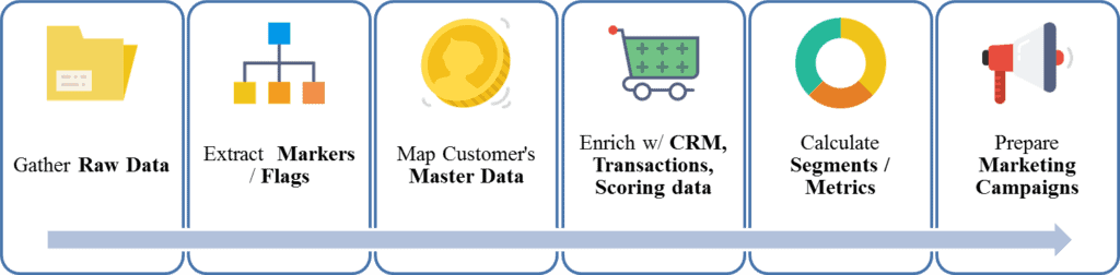
- Gather source data/customer interaction experience
- Extract lots of customer markers/flags
- Map with the client’s master data (identity, contacts, etc.)
- Enrich with CRM / Transactions / Scoring historical data
- Segment database / calculate metrics
- Prepare cross-channel marketing campaigns
Thumbs up, and give me any feedback if you want to hear more about real case studies of applied DWH (data warehousing) / Data Cloud Platforms inside Banking from a Business perspective.
Things have gone wrong – Bottlenecks and Malfunction
A couple of days ago, business users faced a violation of TLA (Time-Level Agreement). The necessary business data was not ready by 9 AM. That consequently created further bottlenecks and delays and resulted in overall process malfunction.
Spheres affected by the issue:
- Business Impact: TLA violation – creates a bottleneck for subsequent operations
- Tech Impact: Excessive System Resource Usage (thus cannibalizing resources from other routines)
The IT team initiated the investigation to address the problem immediately. The closer look resulted in a query posing a severe issue inside Teradata Data Warehouse. The amount of data rose gradually, but the average time to process it increased significantly at one point.
Regarding speed, it takes around 50-60 minutes daily for this query to proceed.
The fundamental question we want to ask is, what is the purpose of this query? What does it do?
Here is a brief description of the business terms:
- Transfer customer interaction experience data from the staging area.
- Map customers to CRM and Payment Card Processing systems through MDM (Master Data Management).
- Remove duplicates; take the customer’s actual ID only.
Technically speaking, several joins with some grouping and filtering are applied.
Eventually, this non-optimal query needs severe treatment. We must find and analyze core causes, implement solutions, and test them to improve performance.
A top-down approach to addressing the problem
First, we need to understand how to approach this kind of problem.
There should be an effective and comprehensive plan to consider everything, see the big picture, identify flaws, and address them best. What would this approach look like?
To find the particular reasons, fix them, and improve the situation, we need to take several steps:
- Analyze the source code
- Gather historical performance metrics
- Examine the execution plan and identify core problems
- Investigate the actual data, its demographics, and distribution
- Propose a viable solution to the issue
- Implement and test it, assess results
Understanding the query purpose
First, we need to understand every query’s purpose from a business perspective. The query should contain no excessive or irrelevant data unless it complies with business needs.
Let us take a more in-depth look at the source code of this particular query. I have left some comments below so you can grasp the general purpose of every stage.
INSERT INTO SANDBOX.gtt_cl_nps_trg_1 (
client_mdm_id,
event_type_id,
event_date,
load_date,
id_target,
load_dt,
tag_v21,
name_product,
tag_v22,
tag_v23)
SELECT
cpty_2.src_pty_cd AS client_mdm_id,
t1.event_type_id,
t1.date_trggr AS event_date,
t1.load_date AS load_date,
t1.id_target AS id_target,
v_curr_dt AS load_dt,
t1.tag_v21,
t1.name_product,
t1.tag_v22,
t1.tag_v23
FROM
(
SELECT
cc.load_date,
cc.trggr_dt AS date_trggr,
cc.client_dk AS id_target,
cc.load_dt AS date_load,
/* 3.2. taking latest party key according to MDM system: */
Max(cpty_1.pty_id) AS pty_id_max,
event_type_id,
cc.tag_v21,
cc.name_product,
cc.tag_v22,
cc.tag_v23
FROM
/* 1. Gathering raw data: */
(SELECT
ncd.load_date,
sbx.load_dt,
sbx.trggr_dt,
sbx.client_dk,
eti.event_type_id,
CASE
WHEN eti.event_type_id IN (’22’, ’23’, ’24’, ’25’, ’26’, ’27’, ’28’, ’29’) THEN sbx.tag_v21
ELSE Cast(NULL AS VARCHAR(200))
end AS tag_v21,
sbx.name_product,
sbx.tag_v22,
sbx.tag_v23
FROM SANDBOX.v_snb_xdl_dm_fvs_nps_sbx sbx
INNER JOIN SANDBOX.gtt_nps_calc_date ncd
ON ( sbx.load_dt = ncd.load_date )
INNER JOIN (
/* … additional data joins … */
) eti
) cc
/* 2. Enriching data with client master key – party external reference: */
LEFT JOIN SANDBOX.v_prd017_REF_PTY_EXTRNL_PTY ref
ON (Cast(cc.client_dk AS VARCHAR(40)) = ref.pty_host_id
AND ref.mdm_system_id=1201)
LEFT JOIN SANDBOX.v_prd017_pty cpty_1 ON ref.pty_id=cpty_1.pty_id
LEFT JOIN SANDBOX.v_prd017_pty_stts stts ON cpty_1.pty_id=stts.pty_id
WHERE stts.pty_stts_id=1401
AND stts.pty_stts_end_dt = DATE’9999-12-31′
/* 3. taking latest party key according to MDM system: */
GROUP BY cc.load_date,
cc.trggr_dt,
cc.client_dk,
cc.load_dt,
cc.event_type_id,
cc.tag_v21,
cc.name_product,
cc.tag_v22,
cc.tag_v23
) t1
/* 3.1. leave one row only with max(party_id) */
LEFT JOIN SANDBOX.v_prd017_pty cpty_2
ON t1.pty_id_max=cpty_2.pty_id
;
All in all, the following steps are performed:
- Getting raw data from view v_snb_xdl_dm_fvs_nps_sbx
- Enriching data with client master key – party external reference
- Removing duplicates – leaving latest entry – max(party_id)
- Inserting result set to be processed on the next steps
Audit Execution Plan and Historical Performance
The best way to analyze historical data on query performance is to use PDCR (Performance Data Collection and Reporting) database and its visually engaging version – Teradata Viewpoint.
Each query executed on RDBMS is stored with crucial metadata such as query text, user, start time, end time, resources consumed, and errors.
So let us dig into some details from the PDCR info database and Teradata Viewpoint Portlet.
What do the performance indicators say?
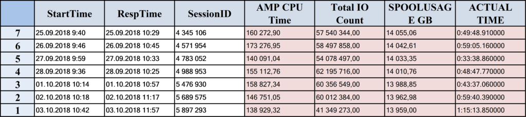
According to the PDCR database query, it utilizes an enormous amount of resources compared to other queries of this particular DataMart:
- CPU Time utilization ~ 160k CPU sec
- Spool Usage ~ 15 TB
- Total IO count ~ 55kk
- It takes around ~ 55 minutes to process on average.
A tremendous amount of memory and CPU seconds are used to store and compute intermediate query results. Further steps take far fewer resources to process. So there are undoubtedly several problems that need to be addressed.
Secondly, here are some pictures from the Teradata Viewpoint Query Spotlight portlet:
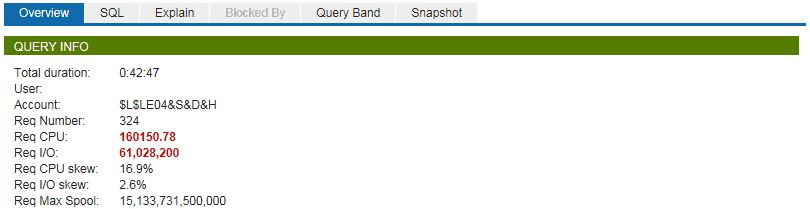
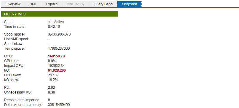
We can see the same performance metrics in a more visually appealing way.
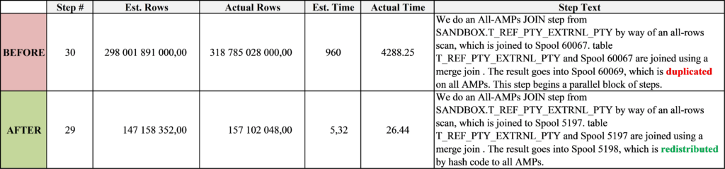
The next step would be examining the actual EXECUTION plan and discovering which steps (operations) result in the most massive load. According to the Explain tab in Teradata Viewpoint Portlet, the most expensive step is one particular JOIN, which took about ~37 minutes (~90% of the time):
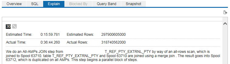
In this step, the following actions are performed:
- We are joining the table of master keys T_REF_PTY_EXTRNL_PTY, with the number of actual rows around 319 billion.
- Duplication of these 319 billion rows to every AMP on the system.
Comprehend Data Demographics
As we identified the most massive operation during that query, let us learn more about our joined data.
Table T_REF_PTY_EXTRNL_PTY is used to accumulate customers’ keys in different banking systems to be matched afterward in the following steps.
That might help determine the customer’s profiles, loans, expenses, preferences, and behavior patterns. This knowledge allows the Bank to offer personalized products and services at appropriate times.
We need to answer several simple questions:
- How many rows are there in a table?
- How many of them do we need?
- How selective is this data by specific columns?
- Which data types are used, and why?
- How is the JOIN performed?
- The table definition goes like this:
CREATE MULTISET TABLE SANDBOX.T_REF_PTY_EXTRNL_PTY , NO FALLBACK ,
NO BEFORE JOURNAL,
NO AFTER JOURNAL,
CHECKSUM = DEFAULT,
DEFAULT MERGEBLOCKRATIO
(
mdm_system_id BIGINT NOT NULL ,
pty_host_id VARCHAR(40) CHARACTER SET Unicode NOT CaseSpecific NOT NULL,
pty_id BIGINT NOT NULL,
deleted_flag CHAR(1) CHARACTER SET Unicode NOT CaseSpecific NOT NULL DEFAULT ‘N’,
action_cd CHAR(1) CHARACTER SET Unicode NOT CaseSpecific NOT NULL,
workflow_run_id BIGINT ,
session_inst_id INTEGER ,
input_file_id BIGINT ,
info_system_id SMALLINT,
pty_extrnl_pty_id BIGINT NOT NULL,
pty_host_id_master_cd CHAR(1) CHARACTER SET Unicode NOT CaseSpecific
PRIMARY INDEX ( pty_id )
INDEX t_ref_pty_extrnl_pty_nusi_1 ( pty_extrnl_pty_id );
So basically, we see that pty_host_id column (customer’s id in different source systems) is VARCHAR(40) type. That is since some systems store customer’s identity with additional symbols like ‘_’, ‘-’, ‘#’, etc. That is why the whole column cannot be stored as a numeric data type.
2. The data distribution by source systems goes like this:
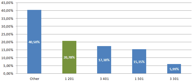
What is most important, we only need a portion of this data! Note that only one specific source system is mapped with the following filtering clause in the source query:
WHERE mdm_system_id=1201
So we don’t need the whole data from the table. We only need around 20% of the data.
Moreover, this data portion is easily cast to numeric data type, joined way easier than a string field. In one of the following chapters, I will show you some benchmarking and comparison of different join types.
- Statistics of data for the optimizer
Ensure statistics are current on tables and columns participating in a query. Statistics is one of the most crucial aspects of the execution plan. Lack of statistics or stale stats may result in Teradata choosing the wrong execution plan and throwing an error, such as ‘No more Spool Space’.
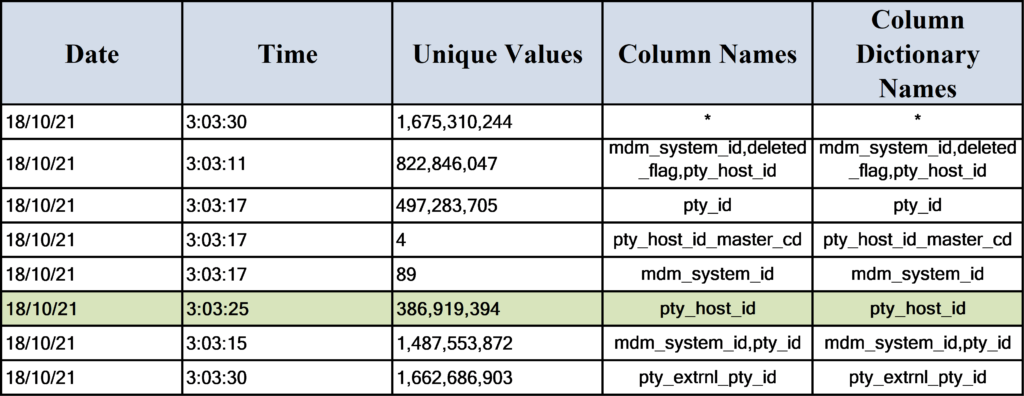
Discover how statistics are collected on a certain table with the SHOW command:
SHOW STATS ON SANDBOX.v_prd017_REF_PTY_EXTRNL_PTY ;
COLLECT STATISTICS
— default SYSTEM SAMPLE PERCENT
— default SYSTEM THRESHOLD PERCENT
COLUMN ( deleted_flag,pty_host_id_master_cd,pty_id ) ,
COLUMN ( mdm_system_id,deleted_flag,pty_host_id ) ,
COLUMN ( deleted_flag,pty_host_id_master_cd ) ,
COLUMN ( pty_id ) ,
COLUMN ( deleted_flag ) ,
COLUMN ( pty_host_id_master_cd ) ,
COLUMN ( mdm_system_id ) ,
COLUMN ( pty_host_id ) ,
COLUMN ( mdm_system_id,pty_id ) ,
COLUMN ( pty_extrnl_pty_id )
ON SANDBOX.T_REF_PTY_EXTRNL_PTY ;
To see the actual stats values and date of gathering, use the HELP command:
HELP STATS ON SANDBOX.v_prd017_REF_PTY_EXTRNL_PTY;
Addressing core problems
Taking everything into account, to improve the query performance, we have to achieve several goals:
- Retrieve only the necessary portion of data from the largest table before joining.
- JOIN on numeric data wherever possible.
- Eliminate the duplication of a colossal amount of data on all AMPs.
- Use the QUALIFY command to exclude unnecessary JOIN, GROUP BY, and apply WHERE (filtering data).
Step #1. Joining the right and easy way
First, let us place the WHERE clause to filter rows we want to JOIN before joining, as we only need around 20% of the whole table.
Secondly, let us cast this data into the numeric data type (BIGINT) to boost performance significantly.
Below I am providing BEFORE and AFTER versions of the source code:
/* BEFORE STATEMENT */
LEFT JOIN SANDBOX.v_prd017_REF_PTY_EXTRNL_PTY ref
ON (Cast(cc.client_dk AS VARCHAR(40)) = ref.pty_host_id
AND ref.mdm_system_id=1201)
/* AFTER STATEMENT */
LEFT JOIN
(SELECT
PTY_HOST_ID
, Cast(Trim(PTY_HOST_ID) AS BIGINT) AS PTY_HOST_ID_CAST
, pty_id
FROM SANDBOX.T_REF_PTY_EXTRNL_PTY
WHERE mdm_system_id=1201
) ref ON cc.id_target = ref.pty_host_id_cast
As a result, we will see that these simple steps will drastically improve the overall query performance and make Teradata optimizer choose a data redistribution strategy instead of duplication (which takes a tremendous amount of time).
Furthermore, I have done some detailed testing on different benchmark kinds of JOIN operations:
- BIGINT = BIGINT
- CAST(VARCHAR as BIGINT) = BIGINT
- CAST(BIGINT as VARCHAR) = VARCHAR
The table with performance metrics is below:
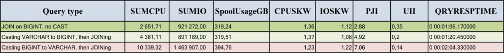
As you can see, the best type of JOIN is on the equality of numeric data types (e.g., BIGINT). This kind of join consumes four times fewer CPU seconds and almost two times fewer IO operations as casting data types and comparing strings sign by sign requires far more CPU resources. Joining on string fields also requires 25-30% more Spool space.
Step #2. QUALIFYing to remove duplicates
Instead of excessive joining, grouping, and applying the aggregate function, we may use a Teradata-specific function to qualify the needed rows. This syntax will help us execute queries more efficient and intelligent way. Let us see how we can do this:
/* BEFORE STATEMENT */
/* 3.3. taking the latest party key according to the MDM system: */
Max(cpty_1.pty_id) AS pty_id_max,
…
/* 3.1. taking latest party key according to MDM system: */
GROUP BY cc.load_date,
cc.trggr_dt,
cc.client_dk,
cc.load_dt,
cc.event_type_id,
cc.tag_v21,
cc.name_product,
cc.tag_v22,
cc.tag_v23
…
/* 3.2. leave one row only with max(party_id) */
LEFT JOIN SANDBOX.v_prd017_pty cpty_2
ON t1.pty_id_max=cpty_2.pty_id
/* AFTER STATEMENT */
QUALIFY Row_Number() Over (PARTITION BY cc.load_date,
cc.trggr_dt,
cc.client_dk,
cc.load_dt,
event_type_id,
cc.tag_v21,
cc.name_product,
cc.tag_v22,
cc.tag_v23
ORDER BY cpty_1.pty_id DESC
) = 1
Applying the QUALIFY clause enables us to leave only one actual data entry per client. Please refer to web resources to learn more about the QUALIFY clause, Row_Number(), and other ordered analytical functions.
Assessing the results
As a result of this analysis, the next step is to implement this new source code, deploy it in testing and production environments, and assess the results.
First of all, how has the execution plan changed?
- The number of actual rows processed has decreased by 2k times! From 319b to 157m.
- The actual time of this step has fallen to 26 seconds compared to 70 minutes before (by 160 times)
- We have eliminated duplication of all rows to all AMPs using this chunk of data instead.
See the actual performance metrics below:
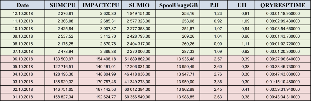
- The total CPU time required for processing has fallen by 60 times because we ensured the best way to join and access data.
- We have saved around 50m IO operations with data blocks by not processing unnecessary data.
- Consequently, the amount of Spool Space used to store intermediate results has decreased by 55 times, from 14 TB to 250 GB.
- Most importantly, our query now takes only around 1 minute to process.
Notice how we improved crucial performance indicators, system resource utilization, and the critical overall time required to process data. This particular query boosted our Data Mart calculation for almost 60 minutes, so our business users get their data in time daily.
Artemiy Kozyr is Data Engineer at Sberbank, Moscow, with a Master’s Degree in CS.
He has five years of Experience in Data Warehousing, ETL, and Visualization for Financial Institutions.
Contacts:
